Software for Windows
Science with your Sound Card!
Features:
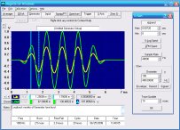
Oscilloscope
Spectrum Analyzer
8-Channel
Signal Generator
(Absolutely FREE!)
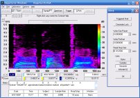
Spectrogram
Pitch Tracker
Pitch-to-MIDI
DaqMusiq Generator
(Free Music... Forever!)
Engine Simulator
LCR Meter
Remote Operation
DC Measurements
True RMS Voltmeter
Sound Level Meter
Frequency Counter
Period
Event
Spectral Event
Temperature
Pressure
MHz Frequencies
Data Logger
Waveform Averager
Histogram
Post-Stimulus Time
Histogram (PSTH)
THD Meter
IMD Meter
Precision Phase Meter
Pulse Meter
Macro System
Multi-Trace Arrays
Trigger Controls
Auto-Calibration
Spectral Peak Track
Spectrum Limit Testing
Direct-to-Disk Recording
Accessibility
Data Logger
Waveform Averager
Histogram
Post-Stimulus Time
Histogram (PSTH)
THD Meter
IMD Meter
Precision Phase Meter
Pulse Meter
Macro System
Multi-Trace Arrays
Trigger Controls
Auto-Calibration
Spectral Peak Track
Spectrum Limit Testing
Direct-to-Disk Recording
Accessibility
Applications:
Frequency response
Distortion measurement
Speech and music
Microphone calibration
Loudspeaker test
Auditory phenomena
Musical instrument tuning
Animal sound
Evoked potentials
Rotating machinery
Automotive
Product test
Contact us about
your application!
Mirror Curve Files
You can create a custom Curve file that exactly compensates or "mirrors" a particular spectrum. This is useful for measuring frequency response using an arbitrary stimulus, or for comparing the response of a unit under test to a reference unit. When the raw response from the system under test has the same spectrum as that used to create the .CRV file, it will appear as a flat line when the .CRV file is applied as a weighting Curve. Deviations from this flat line are thus easy to spot and measure.
For example, the present Pink noise source in the Daqarta Generator does not provide a perfect -3 dB/Octave signal; there is a ripple of +/-0.85 dB in its spectrum. Thus, if you use it as a stimulus to measure the response of a system, and you apply a +3.01 dB/Octave Tilt (which is "perfect") to make it appear flat, the measured response will exhibit this ripple. But if you use a custom Curve file instead, you can get a perfect response measurement.
Or, in a production situation, you may need to insure that the response of each unit matches a reference unit within certain limits. You can use the response of the reference unit to create the .CRV file, then with that as the active Curve you can easily see if production units deviate too far from the now-flat reference line.
The stimulus signal can be just about anything, as long as it is the same in the reference and test conditions. You will need to use spectrum averaging for noise sources, but not for repeating waveforms like bursts, steps, or pulses unless the levels involved are so low that noise is a problem.
Besides production testing, the same approach can be used for production adjustments. If there is some adjustable feature on your Widget that affects the spectrum in a certain test, you can change it dynamically to minimize the deviation from the reference.
To create the .CRV file, the first thing you need is to obtain a spectrum of the signal you want to compensate. For the Pink source, you just view the Generator output directly in Y-log Spectrum mode and average long enough to get a smooth line... or as smooth as you feel you need. Any noise remaining will also appear in the compensated spectrum, so it may be worth waiting a while for a long average.
For a production reference response, you apply your test signal to the standard unit and record the response in the same way you will during production testing.
Now go to the File menu and select Save Y-log Trace as .CAL, .FRD, .CRV, or .LIM File. A dialog will appear with an edit control for Reference Baseline, and a horizontal cursor on the trace will show that value graphically. (The default is the average level between the solid and dotted cursors.)
A single .CRV file can hold data for only one channel, which is shown below 'Channel:' at the top of the dialog. This is also the channel shown on the Y axis, which you can change by toggling off unwanted channel display buttons.
The Reference Baseline value for .CRV files sets the dB level for the flat response line. In general, you will probably want this to be 0 dB, so just enter 0 directly in the control window. Then when you view the corrected response, the Y axis and readouts will show the deviation directly in dB. But you are free to enter any reference value that is relevant to you.
After entering the desired baseline, hit OK and you will see a standard Windows Save As dialog. The default file type is .CAL; you must scroll down and select .CRV files, or the file data will not be mirrored. Enter a file name (or select one you want to replace) and the .CRV file will be created.
To test this file, go to the Spectrum Curves dialog (CTRL+S, C) and click on one of the four wide Weighting Curve File buttons. A standard Windows Open dialog will open, from which you can select the file you just saved. The file name will replace the old button label.
Now, note which channel is active from the reference save and select that channel under the file button you just loaded. The channel trace should instantly become a flat line at the chosen Reference Baseline dB value. This shows that the .CRV file is exactly mirroring the reference response.
If you use 0 dB as the Reference Baseline, the flat line is at the top of the Y axis by default (unless you are using User Units). If a measured response has too large of a peak, it can go off-screen. In that case, you can use SHIFT+PgDn to slide 0 dB down to mid-screen. SHIFT+Home will restore the original unshhifted range top.
You should create the .CRV file at the same sample rate that you will use it, to insure perfect mirror correction. If you use it at a lower rate than recorded, Daqarta will interpolate and the results may still be fairly good. If, on the other hand, you use the file at a higher rate than recorded, Daqarta will attempt to linearly extrapolate the upper values. Since it will base the extrapolation on just the highest two recorded values, the results will usually be terrible above that.
See also Spectrum Curves Dialog, Spectrum Control Dialog
- Back to Standard Weighting Curves
- Ahead to Memory Curves
- Daqarta Help Contents
- Daqarta Help Index
- Daqarta Downloads
- Daqarta Home Page
- Purchase Daqarta
Questions? Comments? Contact us!
We respond to ALL inquiries, typically within 24 hrs.INTERSTELLAR RESEARCH:
Over 35 Years of Innovative Instrumentation
© Copyright 2007 - 2023 by Interstellar Research
All rights reserved