Software for Windows
Science with your Sound Card!
Features:
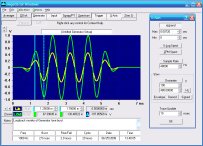
Oscilloscope
Spectrum Analyzer
8-Channel
Signal Generator
(Absolutely FREE!)
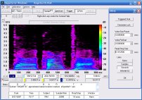
Spectrogram
Pitch Tracker
Pitch-to-MIDI
DaqMusiq Generator
(Free Music... Forever!)
Engine Simulator
LCR Meter
Remote Operation
DC Measurements
True RMS Voltmeter
Sound Level Meter
Frequency Counter
Period
Event
Spectral Event
Temperature
Pressure
MHz Frequencies
Data Logger
Waveform Averager
Histogram
Post-Stimulus Time
Histogram (PSTH)
THD Meter
IMD Meter
Precision Phase Meter
Pulse Meter
Macro System
Multi-Trace Arrays
Trigger Controls
Auto-Calibration
Spectral Peak Track
Spectrum Limit Testing
Direct-to-Disk Recording
Accessibility
Data Logger
Waveform Averager
Histogram
Post-Stimulus Time
Histogram (PSTH)
THD Meter
IMD Meter
Precision Phase Meter
Pulse Meter
Macro System
Multi-Trace Arrays
Trigger Controls
Auto-Calibration
Spectral Peak Track
Spectrum Limit Testing
Direct-to-Disk Recording
Accessibility
Applications:
Frequency response
Distortion measurement
Speech and music
Microphone calibration
Loudspeaker test
Auditory phenomena
Musical instrument tuning
Animal sound
Evoked potentials
Rotating machinery
Automotive
Product test
Contact us about
your application!
EQ_Curve - Example Curves and Parameters
- Introduction
- Standard Weighting Curves
- RIAA Phono Equalization Curves
- Simple Filters
- Complex-Pole Filters
Introduction:
Included here is a collection of EQ_Curve parameter sets, plus images of the resulting curves.
Standard Weighting Curves:
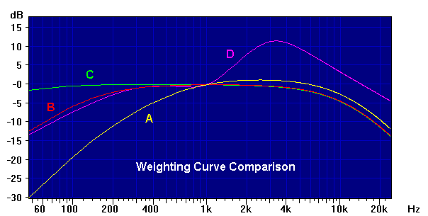
Parameter sets for creation of the A-Weight, B-Weight, C-Weight, and D-Weight curves are given in separate sections below. Usage is discussed in the Standard Weighting Curves topic. All audio weighting curves are normalized to 0 dB at 1000 Hz, by standard convention.
Here is a graphical comparison. Note that B and C are essentially identical above 1000 Hz:
A-Weighting Curve:
Two equivalent A-Weight.CRV parameter sets are presented below. Both use frequencies in radians/second. Along with 4 zeros at DC, A-weighting uses 6 first-order poles. The first parameter set gives the poles as such, while the second capitalizes on the fact that 4 of the 6 comprise two pairs of identical simple poles. It thus gives them as 2nd-order pairs, but with the damping factor set to 2; that makes them non-complex pairs of 1st-order poles. Note that these 4 poles are also the heart of the B-Weight and C-Weight curves below.
A-Weight.CRV - All Simple Poles:
;<Help=H4911
WaitMsg="<<A-Weighting Curve" ;Title
F=1000                     ;Reference freq
UF=2                       ;0=sec, 1=Hz, 2=rad/sec
US=1                       ;-1 = negate curve (inverse curve)

U0=4                       ;DC zeros less DC poles.

U1=6                       ;Number of 1st-order poles and zeros
Buf0[100]=-129.4           ;Neg = pole at 129.4 rad/sec (20.6 Hz)
Buf0[101]=-129.4           ;Second pole at same freq
Buf0[102]=-76655           ;Neg = pole at 76655 rad/sec (12200 Hz)
Buf0[103]=-76655           ;Second pole at same freq
Buf0[104]=-676.7           ;Neg = pole at 676.7 rad/sec (107.7 Hz)
Buf0[105]=-4636            ;Neg = pole at 4636 rad/sec (737.8 Hz)

U2=0                       ;No 2nd order pole or zero pairs
UD=0                       ;0=Re,Im  1=w0,d  2=w0,xi  3=w0^2,d*w0

;---------------------------
A-Weight.CRV - With Pole Pairs:
;<Help=H4911
WaitMsg="<<A-Weighting Curve" ;Title
F=1000                     ;Reference freq
UF=2                       ;0=sec, 1=Hz, 2=rad/sec
US=1                       ;-1 = negate curve (inverse curve)

U0=4                       ;DC zeros less DC poles.

U1=2                       ;Number of 1st-order poles and zeros
Buf0[100]=-676.7           ;Neg = pole at 676.7 rad/sec (107.7 Hz)
Buf0[101]=-4636            ;Neg = pole at 4636 rad/sec (737.8 Hz)

U2=2                       ;Number of 2nd order pole or zero pairs
UD=1                       ;0=Re,Im  1=w0,d  2=w0,xi  3=w0^2,d*w0
Buf0[200]=-129.4           ;Neg = pole at 129.4 rad/sec (20.6 Hz)
Buf0[201]=2                ;Damping = 2 duplicates above pole
Buf0[202]=-76655           ;Neg = pole at 76655 rad/sec (12200 Hz)
Buf0[203]=2                ;Damping = 2 duplicates above pole

;---------------------------
B-Weighting Curve:
The B-Weight.CRV parameters given below use frequencies in radians/second. Note that 4 of the 5 poles are the same as the two pairs of simple poles in the above A-Weight curve. These same 4 poles also appear in the C-Weight curve below.
;<Help=H4911
WaitMsg="<<B-Weighting Curve" ;Title
F=1000                     ;Reference freq
UF=2                       ;0=sec, 1=Hz, 2=rad/sec
US=1                       ;-1 = negate curve (inverse curve)

U0=3                       ;DC zeros less DC poles.

U1=5                       ;Number of 1st-order poles and zeros
Buf0[100]=-129.4           ;Neg = pole at 129.4 rad/sec (20.6 Hz)
Buf0[101]=-129.4           ;Second pole at same freq
Buf0[102]=-76655           ;Neg = pole at 76655 rad/sec (12200 Hz)
Buf0[103]=-76655           ;Second pole at same freq
Buf0[104]=-995.9           ;Neg = pole at 995.9 rad/sec (158.5 Hz)

U2=0                       ;No 2nd order pole or zero pairs
UD=0

;---------------------------
C-Weighting Curve:
The C-Weight.CRV parameters given below use frequencies in radians/second. Note that the 4 poles here also form the cores of the B-Weight and A-Weight curves given above.
;<Help=H4911
WaitMsg="<<C-Weighting Curve" ;Title
F=1000                     ;Reference freq
UF=2                       ;0=sec, 1=Hz, 2=rad/sec
US=1                       ;-1 = negate curve (inverse curve)

U0=2                       ;DC zeros less DC poles.

U1=4                       ;Number of 1st-order poles and zeros
Buf0[100]=-129.4           ;Neg = pole at 129.4 rad/sec (20.6 Hz)
Buf0[101]=-129.4           ;Second pole at same freq
Buf0[102]=-76655           ;Neg = pole at 76655 rad/sec (12200 Hz)
Buf0[103]=-76655           ;Second pole at same freq

U2=0                       ;No 2nd order pole or zero pairs
UD=0

;---------------------------
D-Weighting Curve:
Two equivalent D-Weight.CRV parameter sets are presented below. The first uses frequencies in Hz, and gives the complex 2nd-order poles and zeros as Re,Im pairs. The second uses frequencies in radians/sec and gives the complex parameters in w0^2,d0*w0 format:
D-Weight.CRV - Complex Re,Im Parameters in Hz:
;<Help=H4911
WaitMsg="<<D-Weighting Curve" ;Title
F=1000                     ;Reference freq
UF=1                       ;0=sec, 1=Hz, 2=rad/sec
US=1                       ;-1 = negate curve (inverse curve)

U0=1                       ;DC zeros less DC poles.

U1=2                       ;Number of 1st-order poles and zeros
Buf0[100]=-282.7           ;Neg = Pole at 282.7 Hz
Buf0[101]=-1160            ;Neg = Pole at 1160 Hz

U2=2                       ;Number of 2nd order pole or zero pairs
UD=0                       ;0=Re,Im  1=w0,d  2=w0,xi  3=w0^2,d*w0
Buf0[200]=519.8            ;Pos = Re of complex zero
Buf0[201]=876.2            ;Im of complex zero
Buf0[202]=-1712            ;Neg = Re of complex pole
Buf0[203]=2628             ;Im of complex pole

;---------------------------
D-Weight.CRV - Complex w0^2,d0*w0 Parameters in Rad/Sec:
;<Help=H4911
WaitMsg="<<D-Weighting Curve" ;Title
F=1000                     ;Reference freq
UF=2                       ;0=sec, 1=Hz, 2=rad/sec
US=1                       ;-1 = negate curve (inverse curve)

U0=1                       ;DC zeros less DC poles.

U1=2                       ;Number of 1st-order poles and zeros
Buf0[100]=-1766.3          ;Neg = pole at 1766.3 rad/sec
Buf0[101]=-7288.5          ;Neg = pole at 7288.5 rad/sec

U2=2                       ;Number of 2nd order pole or zero pairs
UD=3                       ;0=Re,Im  1=w0,d  2=w0,xi  3=w0^2,d*w0
Buf0[200]=4.0975e7         ;Pos = Wn^2 of complex zero
Buf0[201]=6532             ;Wn*D of complex zero
Buf0[202]=-3.8836e8        ;Neg = Wn^2 of complex pole
Buf0[203]=21514            ;Wn*D of complex pole

;---------------------------
RIAA Phono Equalization Curves:
These standard weighting curves are useful for testing phono preamplifier equalization. See RIAA Phono Equalization Testing for more details.
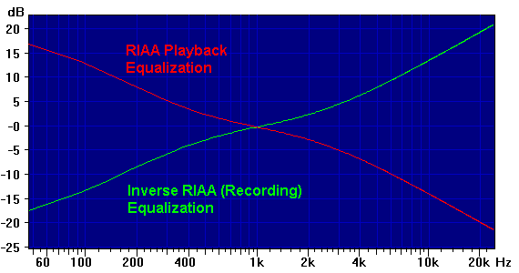
RIAA.CRV:
The red curve above shows the Recording Industry Association of America standard phonograph playback equalization curve. The green curve is the inverse. (See below.)
;<Help=H4911
WaitMsg="<<RIAA Phono Equalization Curve" ;Title
F=1000                     ;Reference freq
UF=0                       ;0=sec, 1=Hz, 2=rad/sec
US=1                       ;-1 = negate curve (inverse curve)

U0=0                       ;DC zeros less DC poles.

U1=3                       ;Number of 1st-order poles and zeros
Buf0[100]=-3180u           ;Neg = Pole at 3180 usec (50 Hz)
Buf0[101]=318u             ;Pos = Zero at 318 usec (500 Hz flatten)
Buf0[102]=-75u             ;Neg = Pole at 75 usec  (2120 Hz low-pass)

U2=0                       ;No 2nd order pole or zero pairs
UD=0                       ;0=Re,Im  1=w0,d  2=w0,xi  3=w0^2,d*w0

;---------------------------
Inv-RIAA.CRV:
By changing the 4th line in the above to US=-1 you can generate Inv-RIAA.CRV, the inverse (negation of dB values) of the RIAA playback curve shown in green in the image above. This is essentially the response of the recording system, which the RIAA playback equalization must compensate to get an overall flat response.
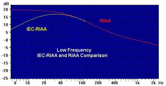
IEC_RIAA.CRV:
This is a modified RIAA playback equalization standard approved by the International Electrotechnical Commission in 1976. Note that this is specified for playback equalization only, to be used with the standard RIAA recording equalization. It is identical to the RIAA curve at frequencies above about 70 Hz. The image below shows the difference at lower frequencies. Note that the frequency axis has been expanded by a factor of 10 using Decimate. See the Display Only section under Using EQ_Curve in the EQ_Curve - Equation-to-Curve Mini-App topic for more information.
;<Help=H4911
WaitMsg="<<IEC-RIAA Phono Equalization Curve" ;Title
F=1000                     ;Reference freq
UF=0                       ;0=sec, 1=Hz, 2=rad/sec
US=1                       ;-1 = negate curve (inverse curve)

U0=1                       ;DC zeros less DC poles.

U1=4                       ;Number of 1st-order poles and zeros
Buf0[100]=-3180u           ;Neg = Pole at 3180 usec (50 Hz)
Buf0[101]=318u             ;Pos = Zero at 318 usec (500 Hz flatten)
Buf0[102]=-75u             ;Neg = Pole at 75 usec  (2120 Hz low-pass)
Buf0[103]=-7950u           ;Neg = Pole at 7950 usec (20 Hz hi-pass)

U2=0                       ;No 2nd order pole or zero pairs
UD=0                       ;0=Re,Im  1=w0,d  2=w0,xi  3=w0^2,d*w0

;---------------------------
Simple Filters:
The following Simple 1st-Order Low-Pass and Simple 1st-Order High-Pass filters can be constructed from nothing more than a resistor and capacitor each, as long as they are driven from a low-impedance source and are driving a high-impedance load. See Filters For Noise Rejection for a discussion.
Simple 1st-Order Low-Pass:
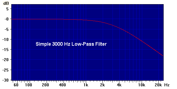
;<Help=H4911
WaitMsg="<<Simple 1st-Order Low-Pass, 3000 Hz" ;Title
F=1                        ;Reference freq
UF=1                       ;0=sec, 1=Hz, 2=rad/sec
US=1                       ;-1 = negate curve (inverse curve)

U0=0                       ;DC zeros less DC poles.

U1=1                       ;Number of 1st-order poles and zeros
Buf0[100]=-3000            ;Neg = Pole at 3000 Hz

U2=0                       ;No 2nd order pole or zero pairs

;---------------------------
Simple 1st-Order High-Pass:
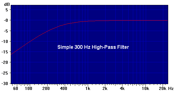
;<Help=H4911
WaitMsg="<<Simple 1st-Order High-Pass, 300 Hz" ;Title
F=24000                    ;Reference freq
UF=1                       ;0=sec, 1=Hz, 2=rad/sec
US=1                       ;-1 = negate curve (inverse curve)

U0=1                       ;DC zeros less DC poles.

U1=1                       ;Number of 1st-order poles and zeros
Buf0[100]=-300             ;Neg = Pole at 300 Hz

U2=0                       ;No 2nd order pole or zero pairs

;---------------------------
Simple Dual 1st-Order Band-Pass:
Note that this is essentially the above 300 Hz high-pass filter followed by the 3000 Hz low-pass. However, you need to either put a buffer amp stage between them (so that the second filter input impedance doesn't load the first), or make sure that the low-pass input resistor is at least 10 times larger than the high-pass resistor, and compute both capacitor values accordingly. See A Simple Band-Pass Filter under the Poles and Zeros subtopic of the EQ_Curve - Equation-to-Curve Mini-App.
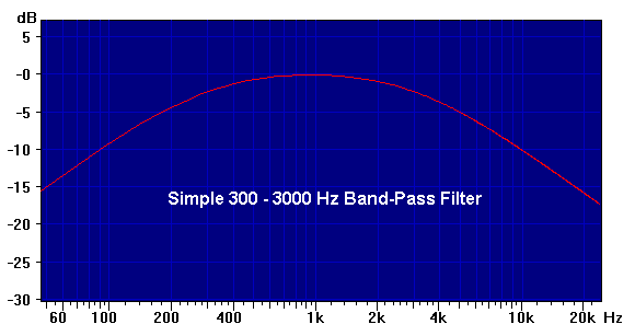
;<Help=H4911
WaitMsg="<<Simple Dual 1st-Order Band-Pass, 300-3000 Hz" ;Title
F=sqrt(300*3000)           ;Reference freq (geometric band center)
UF=1                       ;0=sec, 1=Hz, 2=rad/sec
US=1                       ;-1 = negate curve (inverse curve)

U0=1                       ;DC zeros less DC poles.

U1=2                       ;Number of 1st-order poles and zeros
Buf0[100]=-300             ;Neg = Pole at 300 Hz
Buf0[101]=-3000            ;Neg = Pole at 3000 Hz

U2=0                       ;No 2nd order pole or zero pairs

;---------------------------
Complex-Pole Filters:
The following filters are usually constructed as active filters, which use operational amplifier (op-amp) chips and require operating power. But they are much easier to design and adjust than passive filters, which often require non-standard capacitor and/or inductor values.
A quick Web search on "Active Filter Circuits" will turn up many good documents and sites. The classic introductory text is The Active Filter Cookbook by Don Lancaster, which you can pick up used for a few dollars. Although some of the op-amps he mentions are outdated by modern devices, the basic theory and practical construction tips still hold, and there is plenty of hands-on information to quickly get you building working filters.
Here we focus only on low-pass filters, all designed for a nominal 1000 Hz corner (cutoff) frequency. The following 2-Pole Low-Pass Circuit section shows a basic building block that can be used to create physical filters, but here we deal with the parameters that describe them for EQ_Curve.
All of the low-pass filters presented here use only complex pole pairs. All use frequency in Hz (UF=1 format). The simplest is the 2nd-order (2-pole) Butterworth. There are no zeros at DC and no 1st-order terms, so the relevant part of the EQ_Curve parameter set is:
U2=1                   ;Number of 2nd order pole or zero pairs
UD=1                   ;0=Re,Im  1=w0,d  2=w0,xi  3=w0^2,d*w0
Buf0[200]=-1000        ;Neg = Pole at 1000 Hz
Buf0[201]=1.414        ;Damping factor 'd' for above
Here we have a single pair of poles (since it is a 2-pole filter), so U2=1. The UD=1 format specifies that the first term of each pair will be the pole frequency (in Hz, since UF=1), and the second term will be the damping factor 'd'. We see here that the pole frequency is 1000 Hz (the minus sign indicates that it's a pole, not a zero), and the damping factor is 1.414.
Note that for types other than Butterworth, the poles will not be at the overall cutoff frequency of 1000 Hz. The Bessel poles will be above 1000, and the Chebyshev will be below. Don't worry, they will give the stated 1000 Hz cutoff when both 2-pole sections are used together, with their specified damping factors.
In this and all the filters presented, you can change the cutoff frequency by scaling all pole frequencies: If you want a 2000 Hz cutoff instead of 1000, for example, multiply each pole frequency by 2. Do not change the damping ('d') values.
You can change from low-pass to high-pass in two steps: First, change the number of DC zeros U0=0 to the filter order (U0=2 for the 2nd-order Butterworth, or U0=4 for the remaining 4th-order filters).
Second, divide each low-pass pole frequency into 1000 Hz to get the high-pass equivalent, then multiply by your desired cutoff. This is needed for those filters (other than Butterworth) that have pole frequencies that are not the same as the desired overall corner frequency... it just geometrically mirrors each pole about the target.
For example, the 4th-Order 1 dB Ripple Chebyshev low-pass has poles at 502 and 943 Hz. If you want a 2000 Hz high-pass, the new first pole pair would be (1000 / 502) * 2000 = 3984 Hz, while the second would be (1000 / 943) * 2000 = 2121 Hz.
(Note: The low-pass to high-pass conversion amounts to swapping the positions of tuning resistors R and capacitors C in the following 2-Pole Low-Pass Circuit used for each stage.)
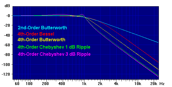
The order of a filter controls how steep the roll-off is well beyond the cutoff; it is 6 * N dB/octave, where N is the order of the filter (number of poles).
The EQ_Curve parameter examples below are all 4th-order, with the exception of a 2nd-order Butterworth for comparison. An even-order filter can be built from a series of 2-pole sections, each a copy of the 2-Pole Low-Pass Circuit but with different values.
You can connect high-pass and low-pass filters in series (cascade) to make a bandpass filter, but only if the passband is fairly wide; if the lower and upper corner frequencies are too close together, the overlapping responses will give poor results.
To determine whether you can use the cascade approach, first find (Fu - Fl) / sqrt(Fu * Fl), where Fu is the upper cutoff frequency and Fl is the lower. If this ratio is approximately 1 or above, a cascade should be fine. If less, a dedicated bandpass design is better... see the Active Filter Cookbook or similar for details.
The response type of a filter (Butterworth, Bessel, Chebyshev) controls the shape near the cutoff, and in the passband itself. It also controls the transient response: Given a step change in a DC input voltage, this refers to how fast the output reaches that voltage, how much it overshoots, and how long it takes to decay back to the final value.
In general, for any given filter order, the sharper you try to make the cutoff, the more transient overshoot and passband ripple. Given a specific goal (such as flattest passband, least transient overshoot, or sharpest cutoff), the filter type can be selected from known characteristics.
Butterworth filters are maximally flat in the passband, but not especially sharp at cutoff. They have a moderate transient overshoot. They are usually the best all-around filter type in most circumstances, unless you are willing to give up passband flatness to achieve some particular goal.
Bessel filters have no transient overshoot at all, but they have a very soft rolloff that extends well into the passband. One virtue for data acquisition is that they also have the least effect on wave shape. While all low-pass filters will soften the edges of a square wave (since they represent high frequencies that are being removed), the more-agressive types also tend to shift the wave's frequency components such that the basic shape is less-representative of the input shape; a square wave typically will have "ringing" after each transient edge.
Chebyshev filters are designed for sharpness at all costs. Besides having the worst transient overshoot and ringing of the types discussed here, they also allow ripples in the passband. By strategic location of a ripple peak right near the corner frequency, they improve the sharpness.
Here is a "big picture" comparison of the frequency reponses of each of the filter types whose parameters are presented below.
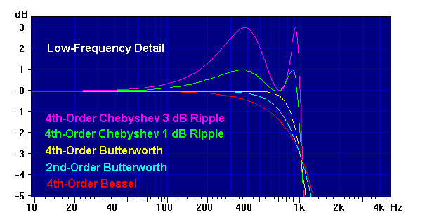
Below is a detail view of the corner frequency region, achieved by setting Decimate to 5x to expand the low frequency range, and by adjusting the vertical axis using PgDn to decrease the dB range, and SHIFT plus PgDn to move the 0 dB point down to mid-screen:
2-Pole Low-Pass Circuit:
Here is a basic circuit for a 2-pole filter that is good for experimentation or limited production:
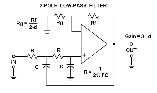
This is called an Equal Value Sallen-Key circuit because both R values are the same, and both C values are the same. To use it, you start by picking capacitor value C, for which you must have two equal-value parts. Then compute the R resistor values from:
R = 1 / (2 * pi * F * C)
Here F is the desired pole frequency. (This will be the same as the corner frequency for Butterworth filters.)
Now select Rf to be somewhere in the vicinity of 2 * R, though this very non-critical. Then using the 'd' damping factor from the parameters for the target filter, compute the value for Rg from:
Rg = Rf / (2 - d)
The gain factor of this 2-pole section will be 1 + Rf/Rg = 3 - d. IMPORTANT: As with all active circuitry, you must make sure that the input signal is not so large that it causes the output to be overdriven. This is usually easy to arrange when the circuit is powered by +/-15 V supplies, but may be more critical with low supply voltages. In some cases you may need an input attenuator to keep the signal within range.
Other topologies have unity gain, but require that the capacitors have specific oddball ratios to get the proper damping. That's harder to arrange than equal values. Resistors may need oddball values, both for setting the pole frequency and the gain of the "equal value" design, but resistors are much cheaper than capacitors, and you can easily use a "trim-pot" for precision gain adjustments.
With the equal-value approach you don't need a huge assortment of capacitor values; factors of 10 are adequate. Typically, 0.001, 0.01, and 0.10 microfarads are all you need to handle the entire audio range. This will result in resistor values in the 10K to 100K range.
For example, with 0.001 microfarad and 10K ohms, the pole frequency will be 15.9 kHz. With 0.10 microfarad and 100K ohms, it will be 15.9 Hz. So, if you are going to experiment, you only need to buy 3 different bags of same-value capacitors, and spend the rest of your budget on op-amps and a big assortment of resistor values, concentrating on the 10K to 100K range.
5% parts tolerance is OK for most 4-pole filters. Don't use old carbon composition resistors (the ones that look like little dark brown cylinders), get carbon film or (better) metal film instead. They have a "dipped" appearance, typically light brown for carbon film and light blue for metal film.
Precision capacitors can be expensive, but since you only need 3 different values, and the exact value isn't important if you have a nice assortment of resistors, you can watch for a sale from a surplus supplier... you might get a bargain on some oddball capacitor value.
Capacitor matching is more important than absolute value, which you can deal with by varying the resistor values. You can use Daqarta's LCR Meter Mini-App to match up pairs of capacitors from your big surplus bag.
The type of capacitor is important, however, especially for temperature stability. In order of best to worst, they are teflon, polycarbonate, polystyrene or polypropolene, polyester (mylar), ceramic, tantalum, and electrolytic. In general, avoid the last 3 completely for filter tuning. Mylar, which is cheap and readily available, may be acceptable for non-critical work.
There are many op-amps that will be acceptable; if you have a favorite on-hand already, you may want to try that first. In general, JFET input types like LF351 or TL081 are a good choice for standard dual-supply circuits, as are the dual op-amp versions LF353 and TL082.
For single-supply op-amps, you will usually have to provide a "ground splitter" consisting of an op-amp buffer and an equal-value voltage divider to set the output to half the the supply voltage. (See the one at the lower left in the External DC-to-AC Modulator circuit diagram.) You then use that op-amp output as the ground in the above circuit.
2nd-Order Butterworth Low-Pass:
Gain factor using the 2-Pole Low-Pass Circuit (above) will be 3 - 1.414 = 1.586.
;<Help=H4911
WaitMsg="<<2nd-Order Butterworth Low-Pass, 1000 Hz" ;Title
F=1                        ;Reference freq
UF=1                       ;0=sec, 1=Hz, 2=rad/sec
US=1                       ;-1 = negate curve (inverse curve)

U0=0                       ;DC zeros less DC poles.

U1=0                       ;Number of 1st-order poles and zeros

U2=1                       ;Number of 2nd order pole or zero pairs
UD=1                       ;0=Re,Im  1=w0,d  2=w0,xi  3=w0^2,d*w0
Buf0[200]=-1000            ;Neg = Pole at 1000 Hz
Buf0[201]=1.414            ;Damping factor 'd' for above

;---------------------------
4th-Order Butterworth Low-Pass:
Gain factor using the 2-Pole Low-Pass Circuit (above) will be (3 - 1.848) * (3 - 0.765) = 1.152 * 2.235 = 2.575.
;<Help=H4911
WaitMsg="<<4th-Order Butterworth Low-Pass, 1000 Hz" ;Title
F=1                        ;Reference freq
UF=1                       ;0=sec, 1=Hz, 2=rad/sec
US=1                       ;-1 = negate curve (inverse curve)

U0=0                       ;DC zeros less DC poles.

U1=0                       ;Number of 1st-order poles and zeros

U2=2                       ;Number of 2nd order pole or zero pairs
UD=1                       ;0=Re,Im  1=w0,d  2=w0,xi  3=w0^2,d*w0
Buf0[200]=-1000            ;Neg = Pole at 1000 Hz
Buf0[201]=1.848            ;Damping factor 'd' for above
Buf0[202]=-1000            ;Neg = Pole at 1000 Hz
Buf0[203]=0.765            ;Damping factor 'd' for above

;---------------------------
4th-Order Bessel Low-Pass:
Gain factor using the 2-Pole Low-Pass Circuit (above) will be (3 - 1.916) * (3 - 1.241) = 1.084 * 1.759 = 1.907.
;<Help=H4911
WaitMsg="<<4th-Order Bessel Low-Pass, 1000 Hz" ;Title
F=1                        ;Reference freq
UF=1                       ;0=sec, 1=Hz, 2=rad/sec
US=1                       ;-1 = negate curve (inverse curve)

U0=0                       ;DC zeros less DC poles.

U1=0                       ;Number of 1st-order poles and zeros

U2=2                       ;Number of 2nd order pole or zero pairs
UD=1                       ;0=Re,Im  1=w0,d  2=w0,xi  3=w0^2,d*w0
Buf0[200]=-1436            ;Neg = Pole at 1436 Hz
Buf0[201]=1.916            ;Damping factor 'd' for above
Buf0[202]=-1610            ;Neg = Pole at 1610 Hz
Buf0[203]=1.241            ;Damping factor 'd' for above

;---------------------------
4th-Order 1 dB Ripple Chebyshev Low-Pass:
Gain factor using the 2-Pole Low-Pass Circuit (above) will be (3 - 1.275) * (3 - 0.281) = 1.725 * 2.719 = 4.690.
;<Help=H4911
WaitMsg="<<4th-Order 1 dB Chebyshev Low-Pass, 1000 Hz" ;Title
F=1                        ;Reference freq
UF=1                       ;0=sec, 1=Hz, 2=rad/sec
US=1                       ;-1 = negate curve (inverse curve)

U0=0                       ;DC zeros less DC poles.

U1=0                       ;Number of 1st-order poles and zeros

U2=2                       ;Number of 2nd order pole or zero pairs
UD=1                       ;0=Re,Im  1=w0,d  2=w0,xi  3=w0^2,d*w0
Buf0[200]=-502             ;Neg = Pole at 502 Hz
Buf0[201]=1.275            ;Damping factor 'd' for above
Buf0[202]=-943             ;Neg = Pole at 943 Hz
Buf0[203]=0.281            ;Damping factor 'd' for above

;---------------------------
4th-Order 3 dB Ripple Chebyshev Low-Pass:
Gain factor using the 2-Pole Low-Pass Circuit (above) will be (3 - 0.929) * (3 - 0.179) = 2.071 * 2.821 = 5.842.
;<Help=H4911
WaitMsg="<<4th-Order 3 dB Chebyshev Low-Pass, 1000 Hz" ;Title
F=1                        ;Reference freq
UF=1                       ;0=sec, 1=Hz, 2=rad/sec
US=1                       ;-1 = negate curve (inverse curve)

U0=0                       ;DC zeros less DC poles.

U1=0                       ;Number of 1st-order poles and zeros

U2=2                       ;Number of 2nd order pole or zero pairs
UD=1                       ;0=Re,Im  1=w0,d  2=w0,xi  3=w0^2,d*w0
Buf0[200]=-443             ;Neg = Pole at 443 Hz
Buf0[201]=0.929            ;Damping factor 'd' for above
Buf0[202]=-950             ;Neg = Pole at 950 Hz
Buf0[203]=0.179            ;Damping factor 'd' for above

;---------------------------
See also EQ_Curve - Equation-to-Curve Mini-App, Macro Examples and Mini-Apps
- Back to EQ_Curve - Equation-to-Curve Mini-App
- Ahead to Thermocouple Macros
- Daqarta Help Contents
- Daqarta Help Index
- Daqarta Downloads
- Daqarta Home Page
- Purchase Daqarta
Questions? Comments? Contact us!
We respond to ALL inquiries, typically within 24 hrs.INTERSTELLAR RESEARCH:
Over 35 Years of Innovative Instrumentation
© Copyright 2007 - 2023 by Interstellar Research
All rights reserved