Software for Windows
Science with your Sound Card!
Gut-Level Fourier Transforms - Part 8:
Unmasking the Aliasing Vampire
Previous Back
By most accounts, aliasing seems to be the scourge of digital data acquisition everywhere, a living curse that walks among innocent data, disguised as a decent citizen, corrupting and contaminating. But before dragging out the sharp wooden stakes of input filters or the garlic of high-speed ADCs, it's worthwhile to understand the demon. Sometimes a little knowledge is all you need to unmask this phantom, and maybe even ward off its evil influence.
Aliasing is a phenomenon related to the sampling of data. To create a digital representation of a waveform, the sampling process takes "snapshots" of the instantaneous value of the wave at regular intervals: the sample rate. Afterward, no information is available about what happened between those samples. If the set of sampled data is to be an accurate representation of the actual waveform, the samples must be spaced closely enough to capture all the significant details.
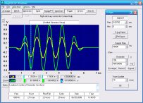
Consider the simple case of a sampled sine wave, as shown in Figure 1. The actual input sine is at 3 kHz, and the solid black squares mark the individual samples that result from sampling at 48 kHz. That sample rate is 16 times the signal frequency, so there are 16 samples per cycle. This allows a perfect reconstruction of the input from the data, as shown by the black curve.
Fig. 1: Aliasing
Note that although the black curve could have simply been drawn "by eye" in a connect-the-dots fashion, in general it requires consideration of the sinusoidal nature of the signal. When there are few samples per cycle, a straight-line approximation would give a poor representation of the waveform. Nevertheless, an FFT analysis could provide the frequency, amplitude, and phase parameters needed to reproduce the input exactly.
However, if the sample rate is reduced by a factor of 18, to 2666.7 Hz, then the new samples (red in Figure 1) coincide with every 18th sample of the original data. Now there is less than one sample per cycle of the input wave. Without knowing the actual frequency of the input, the best-guess fit to this new data would be the curve shown in red. Since this apparent or alias wave takes 4 samples to go through a half cycle, or 8 for a full cycle, we would assume that the input frequency is 2666.7/8=333.3 Hz. The frequency measurement would thus be in error by a factor of nine! And even an FFT would give this same erroneous result... the bite of the alias vampire.
Such alias signals arise whenever the input signal is more than the Nyquist frequency, which is half the sample rate. This is sometimes known as the "folding frequency", because the effect is as though you had folded the true spectrum about that point, causing high frequency components to appear down at the low end of the spectrum. This is actually a pretty good analogy, since it allows you to figure out where those aliased components will appear.
For example, if the Nyquist frequency is 10 kHz (sample rate of 20 kHz), then input components under 10 kHz will appear at their proper locations. But an 11 kHz input will be folded about the 10 kHz point, so it will appear as an alias at 9 kHz. If you sweep the input frequency, a real-time spectrum will show a single peak that moves up until it "hits" the Nyquist frequency and "bounces off". As you continue to increase the input frequency, this peak will now move down toward the low end. The peak will hit zero frequency (DC) when the input is just at the sample frequency, and if you keep sweeping it will bounce back and continue upward.
Given a known input and sample rate, you can figure out where the alias will appear on the spectrum. Divide the input frequency by the Nyquist, and look at the integer portion of the quotient. If it is 0, the input will be shown properly, with no alias. If the integer is odd, you'll get an alias that is coming down from the Nyquist by the fractional part of the quotient (in other words, at the Nyquist frequency times one minus that fraction.) If the integer is even, the alias will be coming up from zero by that fraction of the Nyquist.
In the previous example, 11 kHz/10 kHz=1.10, since the integer is odd we know the alias will be coming down from the Nyquist. Its exact location will thus be (1 - 0.10) × 10 kHz=9 kHz. An input at 23 kHz would give 23 / 10 = 2.30, and since it is even the alias would appear at 0.30 of the Nyquist or 3 kHz.
Note that you can't work this rule backward to find an unknown input frequency given an observed peak: You can't even tell a priori that a peak is an alias, let alone how many times it has been folded over or whether it's on an odd or even fold. That's part of the danger of aliases.
When the input is exactly at the Nyquist frequency, or any multiple of it, the input level is indeterminate. Consider that at half the sample rate there will only be two samples per cycle, and (except for certain synchronous sampling systems) the phase will be unknown. So those two samples could come at the positive and negative peaks, or two zero crossings, or anywhere in between... you just don't know. (That's why spectrum analyzers don't usually show a line corresponding to the Nyquist frequency; it wouldn't have much meaning in most cases.)
The standard defense for warding off aliases is to sample at a higher rate, and if that's not feasible then filter out all signals that could possibly cause aliases, so they are never digitized in the first place. Both of these approaches may have associated costs: Faster ADCs typically cost more, and of course at the higher sample rate you'll acquire more data which will consume more disk or memory space and take longer to analyze.
A conventional anti-alias filter can be even more expensive, depending upon your demands. For example, suppose you want to build the filter in-house using standard active filter designs. The first thing you must determine is the maximum frequency of the valid signals you are trying to analyze, versus the minimum frequency you want to reject. Your filter will need to exhibit unity gain for the valid input, while attenuating the possible aliasing frequency by some specified amount.
Let's say you decide you can tolerate alias components that yield amplitudes no larger than -60 dB relative to the full-scale range of the ADC. Furthermore, in this particular system the highest signal frequency will be 8 kHz, and the lowest possible alias source will be 20 kHz. You plan to set the sample rate to 20 kHz to get a Nyquist at 10 kHz, and use a plain old Butterworth filter to do the alias rejection. But after whipping out your trusty filter design charts, you discover to your dismay that it will take a filter with ten poles just to meet these minimal specs.
Not only will a 10-pole filter require a lot of precision components to achieve the desired response shape, but a 10-pole Butterworth will also have a hefty overshoot in its step response as well. If you can tolerate a 1 dB ripple in the passband, you could use a 9-pole Chebyshev instead, which barely reduces the precision component count and doesn't help the overshoot at all. Conversely, if you want to reduce the overshoot while using a Bessel design, you'll need even more filter poles... a lot more if you want to eliminate overshoot completely. In fact, you may find that your old design charts don't even show Bessel responses beyond 10 poles, and those are down only 15 dB by twice the cutoff, not the required 60 dB... and they have a 2 dB passband droop, to boot.
Starting to feel haunted? There are a couple of approaches you can try. An off-the-shelf filter module may be available that meets your needs, or you may be able to modify your setup slightly to use a readily available module. One alternative that is commonly used in the digital audio world is a sigma-delta ADC (formerly known as delta-sigma) that runs at a much higher input sample rate, but with low initial bit-resolution. This high-speed, low-bits digital stream is then filtered and resampled digitally to yield the final output, with high resolution at a lower sample rate.
Because the initial sample rate is so high, in the hundreds of kilohertz to megahertz range, the Nyquist frequency will be far removed from the region of the input signals. A simple analog filter is all this type of ADC may need at its input, since the real work of anti-aliasing comes during digital resampling to the lower rate. By then the signal is already in digital form, so a very sharp digital filter can be employed right in the ADC chip. In fact, it may be an inherent part of the resampling process, at "no extra charge".
But such sigma-delta converters are rare on laboratory-type boards or single-chip microprocesors, for example. Besides being more expensive initially, they can't be easily multiplexed to handle multiple input channels. So you may want to look harder for a way to use a conventional ADC but still deal with the alias monster.
The simplest solution may be to do nothing at all in hardware, and apply more strategy in the processing. For example, if you are analyzing harmonic distortion components produced by a device under test, you typically have control over the input signal to the system. As mentioned earlier, when the input is moved up in frequency, components that fall between the Nyquist frequency and the sample rate will generate aliases that move down.
These "wrong way" components will show up very plainly when you view a real-time spectrum. You can thus move the input frequency by hand until you are sure which peaks are which, stopping where none of the aliases lands on top of another component. Then you can read the value of each peak directly.
How do you distinguish distortion products that are so high they have folded twice and are moving in the same direction as the input? Easy, if they are harmonic distortion products: Since the Nth harmonic moves N times faster than the fundamental, you'll see large shifts in the positions of such components for small changes in the input frequency. This will immediately tip you off that these are high-order aliases. Then, if you want to know exactly which harmonic is which, you can move the input frequency by one spectral line on the analyzer, and count the number of lines the distortion component moves.
Here the lack of an anti-alias filter is actually an advantage, since it allows you to measure components at higher frequencies. You do, however, need to make sure that the aliased peaks you are trying to read have not been compromised by the sample-hold on the ADC. Typically, the "aperture" on the sample-hold will be significantly narrower than the conversion period, which is what allows this method to work. The simplest way to check that is to feed a known test signal directly into the spectrum analyzer, and see that the peak amplitude doesn't drop as you run the signal over the range of the expected distortion products. Even if it does, you may be able to determine a correction factor for specific test frequencies.
Another approach, not for the faint of heart but definitely possible in certain circumstances, may allow you to make readings even without being able to control the input. If your input signal is a continuous wave, you can sample it in two passes, using slightly different sample rates. Take FFTs of each pass and compare the peaks: A non-aliased signal will show the same apparent frequency in both spectra, although of course it will appear at different spectral lines due to the different sample rates. But an alias will appear to change its apparent frequency as well.
For example, suppose you sample at 20 kHz and 22 kHz. A true 1 kHz component will always show at 1 kHz, but a 19 kHz component will appear at 1 kHz in the first case (having folded at the 10 kHz Nyquist), and at 3 kHz in the second. However, if there are very many peaks to deal with, they can be difficult to keep straight.
There are times when you may want to deliberately run your spectrum analyzer at a low sample rate to get better frequency resolution. Let's say you need 10 Hz resolution and the largest FFT size available is 1024 samples. That would require that the sample rate be no higher than 10240 Hz, with a Nyquist of only 5120 Hz. But you can measure much higher input frequencies by letting them appear as aliases, as long as you know the true frequency to within one Nyquist span.
This is ideal for measuring small frequency drifts, modulation, or amplitude changes in a narrowband signal. However, since the entire input spectrum will be overlapped to appear onto one Nyquist width, it's not the same as a true "zoom" expanded scale feature available on pricier analyzers: You need to make sure that there are no other input features in any frequency range that will confuse the measurement. Nevertheless, this is a handy trick to know for many narrowband applications.
Readers may wish to experiment with aliasing using the author's Daqarta for Windows software that turns your Windows sound card into a full-fledged spectrum analyzer... and much more. You can use the built-in signal generator to allow complete control over signal frequency, and you can monitor the computed values directly to observe aliasing that might otherwise be filtered out by the sound card's anti-aliasing filters if you used a true external signal.
All Daqarta features are free to use for 30 days or 30 sessions, after which it becomes a freeware signal generator... with full analysis capabilities. (Only the sound card inputs are ignored.)
Previous Back
Features:
Oscilloscope
Spectrum Analyzer
8-Channel
Signal Generator
(Absolutely FREE!)
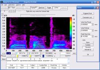
Spectrogram
Pitch Tracker
Pitch-to-MIDI
DaqMusiq Generator
(Free Music... Forever!)
Engine Simulator
LCR Meter
Remote Operation
DC Measurements
True RMS Voltmeter
Sound Level Meter
Frequency Counter
Period
Event
Spectral Event
Temperature
Pressure
MHz Frequencies
Data Logger
Waveform Averager
Histogram
Post-Stimulus Time
Histogram (PSTH)
THD Meter
IMD Meter
Precision Phase Meter
Pulse Meter
Macro System
Multi-Trace Arrays
Trigger Controls
Auto-Calibration
Spectral Peak Track
Spectrum Limit Testing
Direct-to-Disk Recording
Accessibility
Data Logger
Waveform Averager
Histogram
Post-Stimulus Time
Histogram (PSTH)
THD Meter
IMD Meter
Precision Phase Meter
Pulse Meter
Macro System
Multi-Trace Arrays
Trigger Controls
Auto-Calibration
Spectral Peak Track
Spectrum Limit Testing
Direct-to-Disk Recording
Accessibility
Applications:
Frequency response
Distortion measurement
Speech and music
Microphone calibration
Loudspeaker test
Auditory phenomena
Musical instrument tuning
Animal sound
Evoked potentials
Rotating machinery
Automotive
Product test
Contact us about
your application!
Questions? Comments? Contact us!
We respond to ALL inquiries, typically within 24 hrs.INTERSTELLAR RESEARCH:
Over 35 Years of Innovative Instrumentation
© Copyright 2007 - 2023 by Interstellar Research
All rights reserved