Software for Windows
Science with your Sound Card!
Gut-Level Fourier Transforms -
Part 6:
Window Shopping
Previous Next
Having covered the basic theory behind window functions, let's look at various windows and their performance.
By far the most popular window functions are those based upon the raised cosine concept that we discussed last time. These "generalized cosine windows" consist of a DC term (the amount the cosine is raised), the cosine fundamental term, and usually one or more harmonics of that fundamental. The relative values of these terms are adjusted so that the overall function just reaches unity at the center of the data series to which it is applied.
Here are some common window functions, as seen in the time domain:
Fig. 1: Common Window Functions
The Hanning window (sometimes just called Hann) is our simple raised cosine, while the confusingly-similar Hamming is raised a bit more so that it doesn't really go to zero on the ends. These just use the DC and fundamental terms, with no harmonics. The Flat-Top and Blackman windows use a second harmonic term as well, which is so large in the case of the Flat-Top that the curve actually dips below zero (grey line).
There are in fact three different Blackman window functions that appear as the single trace in the figure, since at this resolution they nearly overlap. But these slight differences have a pronouncd effect upon the shape of the spectrum, as we'll see later.
The coefficients for each of these window functions are:
| Window | DC | Fundamental | 2nd Harm |
| Hanning | 0.50 | 0.50 | 0.00 |
| Hamming | 0.54 | 0.46 | 0.00 |
| Blackman | 0.42 | 0.50 | 0.08 |
| Blackman Exact | 0.42659071 | 0.49656062 | 0.07684867 |
| Blackman-Harris | 0.42323 | 0.49755 | 0.07922 |
| Flat-Top | 0.2810639 | 0.5208972 | 0.1980399 |
When those windows are applied to an input signal whose frequency falls midway between two spectral lines (the worst case for leakage), and 1024-point FFTs are taken, the following spectra result:
Fig. 2: Windowed Spectra
The Rectangular "window" is really no window at all, just the normal unwindowed response for comparison. The Blackman ("Bkmn") and Hanning window responses descend into the noise floor of the 16-bit signal. Notice the conspicuous difference between the plain Blackman and the Blackman Exact and Blackman-Harris windows, despite the fact that their function shapes are indistinguishable in Figure 1.
You would choose the Hanning or Blackman windows for measuring very low-level components in the presence of a large input signal. These are particularly useful for distortion measurements, where the distortion components are typically well-removed from the fundamental.
In many cases, the most important feature of a windowed spectrum is how sharply it cuts off near the peak. This becomes critical if you are trying to resolve two input signals that are close together in frequency. Figure 3 shows a greatly expanded view of the central peak area. Note the tick marks along the bottom corresponding to the individual spectral lines.
Fig. 3: Windowed Spectra - Expanded
As you can see from the figures, there are tradeoffs to be made between the peak width, sharpness, and the ultimate low-level floor. What these figures don't show very well is that there are also differences in amplitude accuracy.
Any window function reduces the amplitude of the input signal simply by removing the portions near the end of the sample set. The window function thus introduces a gain factor proportional to the area under the window. In the case of a generalized cosine window, that gain factor is equal to the value of the DC term. This makes sense if you consider that without any DC offset the window would just be a sum of cosine waves. Since those are symmetrical about 0, there would thus be no net area beneath the window. Therefore, any area must come from the offset term.
Consider the simple raised-cosine Hanning window: it has a gain factor (DC term) of 0.5, which requires that all results be multiplied by 2 before display. Spectrum analyzers customarily apply this correction automatically.
That standard correction means that if an input signal falls exactly on a spectral line, the spectrum will show the true magnitude regardless of which window function is selected. But when a signal is between lines, the amplitude may be reduced. We saw last time that with the frequency exactly halfway between lines (the worst case), spectral leakage reduces the unwindowed response by -3.92 dB, to 0.6366 of the true value. The window functions reduce this leakage error, but the amount by which they do so is yet another parameter to juggle when selecting a window.
The following table shows the worst-case error of each window, along with the relative bandwidth of each spectral line (discussed below):
| Window | Error, dB | BW |
| Rectangular | 3.92 | 1.000 |
| Hanning | 1.42 | 1.225 |
| Hamming | 1.78 | 1.168 |
| Blackman | 1.10 | 1.313 |
| Blackman Exact | 1.15 | 1.302 |
| Blackman-Harris | 1.13 | 1.307 |
| Flat-Top | 0.00 | 1.721 |
The amplitude champion here is the Flat-Top, which has essentially a perfect response, in exchange for a broad peak (large BW) and mediocre low-level limit (as seen in Figure 2, where it is the same as Hamming at low levels). This window is ideal for accurate, ripple-free frequency response measurements.
There is another way in which windowing affects amplitude. It broadens the bandwidth of the effective filters for each spectral line. If you use a window with a broadband noise source, this is an issue where there is energy at all frequencies. In the unwindowed (Rectangular) case, adjacent bands overlap in such a way that the total power will be read correctly. The above table shows a BW of 1.000 for this "window." All others are larger.
When the bands are broadened by windowing, the extra overlap means that some of the energy in adjacent bands is "double counted," leading to erroneous higher readings in each. A bandwidth correction factor must be applied in this situation in addition to the amplitude correction discussed above.
Note that BW correction should only be used with broadband signals, not with tonal (line spectrum) inputs. With only the standard amplitude correction and a pure tone input exactly on a spectral line, you will get the same peak height as you select different window types. If you then switch the input to broadband noise, the average level will appear to change with the window type unless you also enable BW correction.
Real-world signals are almost always mixed, since there is always some noise present. The choices you make will depend upon your interests. Consider the output of an oscillator. If you switch on BW correction to read background noise, then the signal peak will be too low. If you leave it off, the noise floor will be too high. The best you can do here is to toggle the BW correction and make dual readings.
With a signal that is entirely broadband, there is no point in using a window at all. Recall that the purpose of the window is to reduce spectral leakage. This is a problem with periodic signals where the analysis length is not an integer multiple of the period. Broadband noise signals are not periodic, so leakage is not an issue.
Transients are another sort of signal that should usually not be windowed, for the same reason as above: they don't represent periodic signals. More importantly, the window may eliminate the most prominent features of the transient, since those are often concentrated near the start. A typical transient, such as an impact, has an abrupt high-level onset, followed by a more gradual decay down to zero. The onset portion would thus be severely or totally removed by the window, which has zero amplitude at its start.
There is also the tail of the transient to consider. The ideal way to handle this is to make sure that your FFT length is long enough to encompass the whole decay region; however, many transients, such as decaying piano notes, don't go neatly to zero in any reasonable length of time. If the decay takes several seconds and you need to use a high sample rate, the number of samples involved may be more than the maximum FFT size of your analyzer.
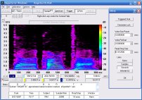
Although you may consider a custom single-ended window that only acted upon the tail, there is a better way: "Slide" the window along the waveform, starting well before the transient, so that at the proper alignment it will be in the middle of the window. This method allows you to visualize the spectrum of the transient as it evolves over time. One standard way to display this spectrum vs. time information is the spectrogram, which we'll cover next time.
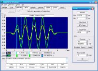
Readers can experiment with window functions using the author's Daqarta for Windows software that turns your Windows sound card into a full-fledged spectrum analyzer... and much more. The built-in signal generator can create both waveform and noise signals of many types, which allows you to evaluate window performance on mixed signals. In addition, you can produce a wide variety of transient signals.
Previous Next
Features:
Oscilloscope
Spectrum Analyzer
8-Channel
Signal Generator
Spectrogram
Pitch Tracker
Pitch-to-MIDI
DaqMusiq Generator
(Free Music... Forever!)
Engine Simulator
LCR Meter
Remote Operation
DC Measurements
True RMS Voltmeter
Sound Level Meter
Frequency Counter
Period
Event
Spectral Event
Temperature
Pressure
MHz Frequencies
Data Logger
Waveform Averager
Histogram
Post-Stimulus Time
Histogram (PSTH)
THD Meter
IMD Meter
Precision Phase Meter
Pulse Meter
Macro System
Multi-Trace Arrays
Trigger Controls
Auto-Calibration
Spectral Peak Track
Spectrum Limit Testing
Direct-to-Disk Recording
Accessibility
Data Logger
Waveform Averager
Histogram
Post-Stimulus Time
Histogram (PSTH)
THD Meter
IMD Meter
Precision Phase Meter
Pulse Meter
Macro System
Multi-Trace Arrays
Trigger Controls
Auto-Calibration
Spectral Peak Track
Spectrum Limit Testing
Direct-to-Disk Recording
Accessibility
Applications:
Frequency response
Distortion measurement
Speech and music
Microphone calibration
Loudspeaker test
Auditory phenomena
Musical instrument tuning
Animal sound
Evoked potentials
Rotating machinery
Automotive
Product test
Contact us about
your application!
Questions? Comments? Contact us!
We respond to ALL inquiries, typically within 24 hrs.INTERSTELLAR RESEARCH:
Over 45 Years of Innovative Instrumentation
© Copyright 2007 - 2026 by Interstellar Research
All rights reserved