Software for Windows
Science with your Sound Card!
Features:
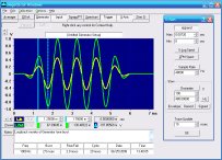
Oscilloscope
Spectrum Analyzer
8-Channel
Signal Generator
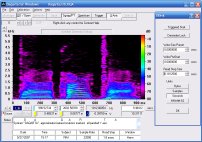
Spectrogram
Pitch Tracker
Pitch-to-MIDI
DaqMusiq Generator
(Free Music... Forever!)
Engine Simulator
LCR Meter
Remote Operation
DC Measurements
True RMS Voltmeter
Sound Level Meter
Frequency Counter
Period
Event
Spectral Event
Temperature
Pressure
MHz Frequencies
Data Logger
Waveform Averager
Histogram
Post-Stimulus Time
Histogram (PSTH)
THD Meter
IMD Meter
Precision Phase Meter
Pulse Meter
Macro System
Multi-Trace Arrays
Trigger Controls
Auto-Calibration
Spectral Peak Track
Spectrum Limit Testing
Direct-to-Disk Recording
Accessibility
Data Logger
Waveform Averager
Histogram
Post-Stimulus Time
Histogram (PSTH)
THD Meter
IMD Meter
Precision Phase Meter
Pulse Meter
Macro System
Multi-Trace Arrays
Trigger Controls
Auto-Calibration
Spectral Peak Track
Spectrum Limit Testing
Direct-to-Disk Recording
Accessibility
Applications:
Frequency response
Distortion measurement
Speech and music
Microphone calibration
Loudspeaker test
Auditory phenomena
Musical instrument tuning
Animal sound
Evoked potentials
Rotating machinery
Automotive
Product test
Contact us about
your application!
Macro Math Functions
- Introduction
- Logarithmic and Exponential Functions
- Trigonometric Functions
- Hyperbolic Functions
- Integer and Sign Functions
- Unsigned Integer to Float Function
- Integer To String Function
- Bit Count Function
- Byte Swap Functions
- Random Value Functions
- Limit Functions
- Color Function
- Channel Status Function
- Data Point Functions
- Sigma (Summation) Functions
- Peak Functions, Buf0-Buf7
Introduction:
A macro math function consists of a keyword followed by an argument (value or expression in parentheses), such as sqrt(A^2 + B^2). In the tables that follow, functions will be shown wih empty parentheses, as in sqrt().
Some special functions take two arguments, and some can take either one or two arguments. If two arguments are given, they are separated by a comma.
Note that math functions may not be used in string expressions, only math expressions. For example, you may not use Msg="Number = " + rand(0,100). Instead, you can use A=rand(0,100) followed by Msg="Number = " + A.
Logarithmic and Exponential Functions:
    log()      Natural logarithm (base e)
    ln()       (Same as above)
    log10()    Common logarithm (base 10)
    log2()     Base-2 logarithm
    exp10()    Raise 10 to a power
    exp()      Raise e to a power
    exp2()     Raise 2 to a power
    sqrt()     Square root
Note that the logarithm of zero or a negative number is undefined, and will return an error value equal to the maximum negative for the type of variable in use. There is no such issue with exponentials or square roots, although the square root of a negative number will be positive.
Trigonometric Functions:
All angles are in radians. There are 2 * pi radians in a circle of 360 degrees, so to convert radians to degrees, multiply by 360 / (2 * pi). To convert degrees to radians, multiply by 2 * pi / 360.
    sin()      Sine of an angle
    cos()      Cosine of an angle
    tan()      Tangent of an angle
    asin()     Arc sine; angle whose sine is ()
    acos()     Arc cosine; angle whose cosine is ()
    atan()     Arc tangent; angle whose tangent is ()
Note: The atan() function can accept either one or two arguments. If two arguments are given they are assumed to be in the form atan(Y,X), which is the angle whose tangent is Y / X. In the C programming language this would be called atan2. This two-argument form is preferable where possible, because it does not have the divide-by-zero issues that would result from pre-dividing Y / X, and because it can can keep track of the sign of the resultant angle over all 4 quadrants
Hyperbolic Functions:
    sinh()     Hyperbolic sine
    cosh()     Hyperbolic cosine
    tanh()     Hyperbolic tangent
    asinh()    Hyperbolic arc sine
    acosh()    Hyperbolic arc cosine
    atanh()    Hyperbolic arc tangent
Integer and Sign Functions:
    abs()      Absolute value
    sgn()      Sign of () = 0, +1, or -1
    sign()     Sign of () = +1 or -1
    int()      Integer part of (), no rounding
    fix()      As above, but negatives truncate toward 0
    cint()     Rounds away from 0 if abs(fraction) >= 0.5
    ceil()     Rounds to next-highest integer
Examples:
  A      abs(A)    sgn(A)  sign(A)   int(A)    fix(A)    cint(A)    ceil(A)
  3.7     3.7       1.0      1.0      3.0       3.0        4.0       4.0
  3.1     3.1       1.0      1.0      3.0       3.0        3.0       4.0
  0       0         0        1.0      0         0          0         0
 -3.1     3.1      -1.0     -1.0     -4.0      -3.0       -3.0      -3.0
 -3.7     3.7      -1.0     -1.0     -4.0      -3.0       -4.0      -3.0
Note: If you are familiar with the C programming language, Daqarta's int() is equivalent to C's floor(). Similarly, fix() is equivalent to trunc().
Unsigned Integer To Float Function:
uns(UA)
Daqarta's integer and fixed-point variables are assumed to be signed values in the range of 2^31-1 to -2^31. However, you may encounter unsigned 32-bit integers from such sources as Arduino boards. If an unsigned integer is less than 2^31 there is no problem, but if it is larger it will be treated as a negative value by Daqarta. To avoid this issue, you can use the uns() function to force it to be treated as an unsigned float variable.
For example, if you use UA=Port?4 to read a 4-byte unsigned Arduino 'long' value into integer UA, you can follow it with A=uns(UA) to make sure that floating point variable A is properly unsigned over the full 32-bit range.
Integer To String Function:
str(UI)
This function accepts an unsigned 32-bit binary integer in UI and returns the equivalent ASCII string. The returned value is always 4 ASCII characters, padded with zeros as needed. For example, if UI = 32 then str(UI) = h30303332 = "0032".
Note that the 4-character result limits the useful range to 0-9999. Larger values will be truncated after conversion. For example, if UI = 123456789 then str(UI) will be h31323334 = "1234".
A typical use is to build up a string-equivalent integer. For example, UA="Nu" << 16 + (str(UI) & hFFFF) will give "Nu08" if UI is 8, "Nu16" if 16, "Nu32" if 32, etc.
Bit Count Function:
bcnt(X) returns the number of bits set in the integer representation of (X), which may be a variable or expression. Values are rounded to 32-bit integers before evaluation; a value of -1 always returns 32.
Byte Swap Functions:
Values in the x86-compatible family of processors used by Windows are known as "little-endian". In the 4 bytes that make up a 32-bit integer, the least-significant byte appears first in memory, followed by increasingly significant bytes at higher memory locations. Consider the hexadecimal value A0A1A2A3; the bytes would be stored in this order in memory: A3, A2, A1, A0. Other processors may be "big-endian", such that the bytes are stored in the order that humans would write them down: A0, A1, A2, A3.
bswp() and bswp2 simplify handling of binary files that use the big-endian format, such as .JPG image files. (See, for example, the use of bswp2 by the _Music_JPG subroutine of the Music_from_Anything macro mini-app.)
bswp(UX) reverses the order of the 4 bytes that make up 32-bit integer UX, so A0A1A2A3 would become A3A2A1A0.
Note: If a float variable such as X or a fixed-point varible such as VarX contains a fractional part, the 32-bit integer and 32-bit fraction parts are handled separately and recombined; there is no swapping between the integer and fraction parts. For example, if the value in hex was 12345678.9ABCDE00, after bswp the value would be 78563412.00DEBC9A.
bswp2(UX) is a special form for 16-bit values that have been read into a 32-bit integer. The hex value A0A1 would be stored in UX as 0000A1A0, such that the above bswp(UX) would give A0A10000, whereas bswp2(UX) returns the desired 0000A0A1.
Note that if you use bswp2 with a full 32-bit value, the high 16-bit byte pair and the low 16-bit byte pair will be swapped separately. Hex A0A1A2A3 would become A1A0A3A2. With floats like X or fixed-point variables like VarX, the integer and fraction parts are also handled separately, as noted for bswp above, but now bswp2 would convert 12345678.9ABCDE00 into 34127856.BC9A00DE.
Random Value Functions:
    rand()     Random 64-bit value between specified limits
    rnd()      Random 32-bit value between specified limits
    Posn?R     Random 32-bit integer using above generator
    Posn?r     Read seed of above generator
    Posn#r     Set seed of above generator
rand(A,B) returns a random floating-point value having 64-bit resolution between A and B, where A and B may be constants, variables, or expressions. If only one parameter is given, the other is assumed to be 0.
rnd(A,B) behaves the same way, but uses a simpler 32-bit linear congruential generator. This reduced resolution will rarely be significant, but this generator has the advantage that it is simple to repeat a sequence of values by setting the same seed with Posn#r. You can also read the current seed via Posn?r and save it to a fixed-point variable Var0-Z to continue the current sequence in the next Daqarta session. You can even experiment with different generator parameters... see the Advanced Users section at the end of Mouse and Miscellaneous Position Macros.
You can use Buf0="<r(A,B)" to effectively apply the rnd(A,B) math function to fill all 1024 elements in an array.
The rnd() generator can be invoked from a MIDI Changes script via ?r(min,max). It is identical to but independent from the default ?(min,max) MIDI random generator when the latter is in pseudo-random mode via the ?x=0 command.
See Random Macro Values for a discussion of use.
Limit Functions:
    lim(X,min,max)   Limit X to given range.
    lim(X)           Limit X to preset range.
    limx(X,min,max)  Limit X to given range, else 0.
    limx(X)          Limit X to preset range, else 0.
    limr(X,min,max)  If X is outside range, roll to other end.
    limr(X)                As above but with preset range.
    Lim=max          Preset max limit.  (Also Lim#M=max.)
    Lim#m=min      Preset min limit.
    Lim              Returns preset max limit.  (Also Lim?M.)
    Lim?m            Returns preset min limit.
lim(X,A,B) limits X to values in the range between A and B. The order of A and B does not matter; either can be the maximum or minimum. Values outside the range are limited to the maximum or minimum.
lim(X) works just like the above, except that the limits must be set ahead of time with the Lim command (see below).
limx(X,A,B) behaves like lim(X,A,B) except that values outside the specified range are limited to zero.
limx(X) works just like the above, except that the limits must be set ahead of time with the Lim command.
limr(X,A,B) limits X to the specified range, but if it is above the range it "rolls" to the minimum, and if it is below it rolls to the maximum.
limr(X) works just like the above, except that the limits must be set ahead of time with the Lim command.
Lim (note case) is a command, not a function. It sets the limits for the above lim() and limx() functions. Lim=A or Lim#M=A sets the maximum limit to A. Lim#m=B sets the minimum limit to B. It doesn't matter if the "minimum" is greater than the "maximum", since the lim() and limx commands re-order the limits in operation.
These preset limits are only changed by the Lim commands. They are completely independent of the limits that may be explicitly specified directly in the lim() or limx() functions.
You can read the preset limit values as needed. Lim or Lim?M returns the maximum, and Lim?m returns the minimum.
Note: If you set both limits to the same value, either explicitly in the function or preset via Lim, the lim() function will always return that value. However, limx() will return that value only if the input variable is exactly equal; otherwise it returns 0. This can be useful with integers, but with real numbers there may be tiny rounding or trucation errors in calculation results (as small as one part in 2^64) that make this method unreliable.
In such cases, you should convert to an integer first. (See Integer and Sign Functions, above.) You can handle a desired number of decimal places by pre-multiplying by that number of decades, then converting to an integer. For example, instead of limx(X,123.456,123.456) to exclude all values of X other than 123.456, you can use limx(int(1000*X),123456,123456) / 1000.
Color Function:
    colr(Hue,Tint)
    colr(Hue)
This function returns a 24-bit ColorNum value in the range of 0 to 0xFFFFFF (16777215). The purpose of this function is to allow one or two variables to smoothly control color, which involves 3 separate color components: Red, Green, and Blue.
Color numbers used by Windows are of the form 0x00bbggrr, where 'rr' is the low byte and controls the amount of red, 'gg' is the next-highest byte and controls green, and 'bb' is blue. A single control (such as a slider) that covers this entire range does not give a useful color response, since the settability of such a control is far too coarse. Slight twitches result in huge and seemingly-random color jumps.
Even if resolution was not an issue, a linear control would not give a user-friendly response. As the control smoothly increased from 0 (pure black) it would hit pure red at 255 (0X0000FF). But the very next step would be pure black with one unit of green (0x000100), indistinguishable from black. Continued increase would again increase red to maximum, then drop back to black with 2 units of green. And so on.
The colr() function resolves the resolution issue and also arranges the colors into a conventional color wheel.
(Note that a visible-light spectrum contains only colors that can be perceived with single-wavelength light, as seen in a rainbow, or by passing white light through a prism. It runs from red through yellow, green, cyan, and blue, but does not include magenta. The brain perceives magenta when both red and blue receptors are stimulated, but not green.)
As Hue (which may be a simple value, variable or expression) varies from 0-1535 the returned color number varies from pure red through all the fully-saturated colors of the color wheel and back to red.
Hue values from 1536 to 1791 vary from black through shades of gray (all color components equal) to white.
The Tint value, which may be from -255 to +255, is then added to each of the three color components of the saturated color number. No component is allowed to exceed 255 or go lower than 0. The effect of this is that positive Tint values move the effective color toward white (washed out) and negative values move the color toward black.
You can omit the Tint value to obtain fully-saturated colors from a single Hue variable.
A typical use for this function is shown in the Line Color control of the Diff_Chan macro mini-app. It is also used in the Input Color Mod function implemented in _Liss_Task of the Lissajous mini-app, and in the color button of the FFT Filter mini-app.
See Mouse and Miscellaneous Position Macros for an example of a Task that allows the mouse position to change trace color, where Hue is controlled by horizontal position and Sat by vertical position.
See also the _Color_Tint macro to lighten or darken an existing color.
Channel Status Function:
chan() Input or output channel state
chan(C) returns 1 if the channel specified by C is active, else 0. C may be a constant, variable, or expression, which is rounded to an integer to get the channel number whose status is to be tested:
    0 = Left In
    1 = Right In
    2 = Left Out
    3 = Right Out
Any value outside this range will return 0. A channel is considered to be active if there are data values available, even though its display button may be off.
This function is especially useful with Data Point Functions (below) and Sigma (Summation) Functions, which require a valid channel number. It can be used by Custom Controls to restrict selection to only active channels, such as for use with a Custom Meter that uses the sSig() function. (The custom control would set the validated channel for use via the Channel Select Ch command.)
Data Point Functions:
    Wv()       Waveform data value for channel and index
    Sp()       Spectrum magnitude for channel and index
    Av()       Averager data value for channel and index
These functions return single values from internal Daqarta arrays. There is a separate function for each type of array: Wv() for waveform, Sp() for Spectrum, and Av() for Averager array data.
All data point functions use the form Wv(C,N) to return the Nth data point of channel C, where N and C may be constants, variables, or expressions. N is limited to 0-1023 or 0-512, depending on mode. (See individual function descriptions below.) Channels are limited to 0-3:
    0 = Left In
    1 = Right In
    2 = Left Out
    3 = Right Out
The data point functions also have a single-argument form Wv(N) which requires that the channel be previously set via the Channel Select macro Ch.
Returned data point values are effective ADC or DAC counts, such that +/-32767 represents a full-scale signal. To convert to volts or User Units, see Macro Data Unit Conversions. Exceptions: For Histogram and PSTH averages, Av() return values are percentage of "hits" on each histogram bin, scaled such that 32768 is 100%.
TIP: You can use CursN to get the N index from the current solid cursor position, or CursDotN for the dotted cursor. For example, A=Wv(0,CursN) sets variable A to the Left In waveform data point that is under the cursor. Note that the index values returned by CursN and CursDotN are mode-specific. In waveform display mode they can range from 0-1023, while in Spectrum mode they only range from 0-511.
Wv(C,N) returns the Nth instantaneous (not averaged) waveform data point of channel C. Index N is limited to 0-1023. You can use Wv() in any display mode, even Spectrum or Spectrogram, since those both start out with raw waveform data.
Sp(C,N) is similar to Wv(), but returns the Nth instantaneous spectrum magnitude data point of channel C. Index N is limited to 0-511. Results are only valid if Spectrum or Spectrogram modes are active.
Av(C,N) returns the Nth averaged data point of channel C for the current (wave or Spectrum) mode. The result is only valid for a running or completed Average. For wave mode, data point index N is limited to 0-1023, except for Histogram averages where it is limited to 0-511. In Spectrum mode it is always limited to 0-511.
Sigma (Summation) Functions:
    wSig()     Waveform Sigma (RMS) between indices
    BwSig()    Buf0-7 waveform Sigma between indices
    sSig()     Spectrum Sigma (magnitude) between indices
    BsSig()    Buf0-7 spectrum Sigma between indices
The summation functions operate on internal Daqarta arrays, including macro arrays Buf0-Buf7. Unlike the previous data point functions, summation functions operate on a range of index values. They all use the general form of wSig(M,N), where index values M and N may be constants, variables, or expressions.
These functions behave like the Sigma display of the cursor readouts, which depends upon display mode. The 'w' versions wSig() and BwSig() operate on waveform data, while the 's' versions sSig() and BsSig() operate on spectrum data.
The channel number must be set ahead of time via the Channel Select command Ch. Channels are limited to 0-3 for wSig() and sSig(), as for the above data point functions. BwSig() and BsSig() operate on Buf0-Buf7 data arrays, where the "channel" is really the buffer number 0-7.
The waveform functions wSig() and BwSig() compute the effective RMS (Root Mean Square) of the raw data between (and including) the index values. Each raw data value is squared and added to a total, the final total is divided by the number of values to yield a mean, and the square root of the mean is returned.
This is the same fundamental operation as performed by the waveform cursor Sigma mode or the RMS mode of the Voltmeter. Unlike the Voltmeter, however, you can specify a specific region of the waveform, and unlike the Sigma mode you don't have to move the cursors to select that region. (But you can use CursN and CursDotN as indices to get that same function.) You can easily find separate RMS values for different parts of a waveform.
You can also use Posn?S to find the number of samples to use for waveform-synchronous RMS measurements. See the Macro Notes section under Voltmeter RMS.
As with the above data point functions, returned Sigma values are effective ADC or DAC counts, such that 32767 represents a full-scale (zero-to-peak) signal. However, note that RMS values are typically less (sometimes much less) than full scale. For example, a full-scale sine wave will have an RMS value equal to 0.707 times the peak, or about 23170 here. To convert to RMS volts or User Units, see Macro Data Unit Conversions.
wSig() index values are limited to 0-1023. The current instantaneous waveform data is used to compute the RMS value unless a waveform average is running or done, in which case Averager data is used.
For Histogram averages, wSig() index values are limited to 0-511 (corresponding to the 512 "bins" of the Histogram display). The function returns a simple summation of the contents of the included bins, scaled to read in percent. This gives the percent of samples whose amplitudes fall between the index values, inclusive, so a value of 100.000 means that all the samples in the waveform are included.
For Post-Stimulus Time Histogram (PSTH) averages, wSig() index values are limited to 0-1023. A simple summation of PSTH bins is used, such that the return value indicates the percent of averager frames with events above the PSTH threshold at each time point. In an idealized case, if the threshold is set to zero and the signal is a pure sine wave, the PSTH display would show spikes of 100% at each positive-going zero crossing. If the wSig() indices surround one such zero crossing spike, the function would return a value of 100.000. (If there are multiple cycles in the waveform display and more than one spike is included between the indices, the return value would be a multiple of 100.)
In a more typical PSTH case, the signal will have noise or jitter which causes the threshold to be reached a little earlier or later on different repetitions. Instead of a single 100% spike at each zero-crossing, there would be a distribution of spikes that together should total 100%. wSig() can give the total percent of spikes at any given distance from a chosen target value. By varying the index values, you can generate a cumulative distribution curve.
You can use wSig() in any display mode, including Spectrum and Spectrogram, but only instantaneous waveform data will be used in those cases.
BwSig(M,N) returns the effective waveform RMS value between index numbers M and N, inclusive, for the selected macro array Buf0-Buf7. Index values are limited to 0-1023. The buffer number (0-7) must be preset via the Ch Channel Select command. BwSig() behaves like wSig(), except it is completely independent of the current display mode or Averager state. In particular, it does not provide special summation-only handling for Histogram or PSTH averages. If you copy Linear or Exponential averaged data to a buffer and apply BwSig(), you will get the same result as if you had used wSig() directly on the averaged data. You will not get equivalent results for Histogram or PSTH data.
The Spectrum summation functions sSig() and BsSig() compute the effective magnitude of the raw spectrum data between (and including) the index values. They compute the square root of the sum of squares of the magnitudes at each included spectral line. (Unlike waveform RMS, there is no "Mean".) The result is the "effective" amplitude of a sine wave that has the same energy as the included components. See the Sigma topic for an example.
The returned value can equal or even exceed the full-scale (zero-to-peak) value of 32767. For example, a full-scale square wave will return a value of 1.414 times this if the indices include the full spectrum. (If you convert this "effective sine wave" amplitude to RMS by multiplying by 0.707, you will see that the RMS value of a square wave is the same as its amplitude. This makes perfect sense, since the RMS value is the equivalent DC value that would provide the same heating energy in a simple resistance; a square wave is essentially a DC value switched between positive and negative, both of which heat a resistor equally well.)
sSig(M,N) returns the effective Spectrum magnitude value between indices M and N, inclusive, for the selected channel. Index values are limited to 0-511, and channels (set via the Ch Channel Select command ahead of time) are limited to 0-3. Results are only valid if Spectrum or Spectrogram modes are active, otherwise the return value is 0. If a Spectrum Average is running or done the averaged magnitude values are used, otherwise the current instantaneous spectrum is used.
BsSig() behaves just like sSig() except that it works on macro data arrays Buf0-Buf7, so you must pre-set the desired "channel" to 0-7 with the Ch Channel Select command. Also, this function may be used in any display mode, as long as the Buf0-7 array holds raw FFT spectrum data. It does not work with Spectrum Average data, even if you copy it to the buffer ahead of time.
Note that although both sSig() and BsSig() only allow indices in the 0-511 range, they are really working on arrays of 1024 values. The raw instantaneous FFT spectrum consists of 512 pairs of values called "Real" and "Imaginary" (Re and Im), each pair representing one of 512 spectral lines designated 0-511. See Macro Arrays Buf0-Buf7 for information on how to access individual Re and Im values for instantaneous spectra. (A Spectrum Average, however, consists of only 512 average magnitude values, no separate Re and Im values.)
Peak Functions, Buf0-Buf7:
pkB(N) returns the most-positive value in the BufN array, where N = 0-7. After this operation the index (0-1023) of the peak will be in read-only variable Posn?p.
pkb(N) is identical to the above, but only scans the first 512 points in the designated BufN array. This is useful for scanning spectrum magnitudes or curves that only occupy the lower 512 points, since it ignores any remains of prior 1024-point data in the upper half.
pkB(N) and pkb(N) only find the most-positive value. (But see below.) To find the most-negative, negate the array first with Buf0="<~(0)", then use the pkB() or pkb() function. Negate the peak to get its original sign.
Alternatively, you could take the absolute value of each Buf0 element using Buf0="<|", then use the pk function to find the largest peak regardless of sign.
The above peak functions allow you to specify the BufN array number via a variable or expression. If you don't need that ability, and you want the peak of all 1024 points, you can use an explicit BufN math operation to return the positive or negative peak. For example, X=Buf0?p sets X to the most-positive peak in Buf0 (identical to X=pkB(0)), while X=Buf0?n sets the most-negative peak.
See also Macro Arrays Buf0-Buf7, Macro Overview
- Back to Macro Expressions and Operators
- Ahead to Macro Variables
- Daqarta Help Contents
- Daqarta Help Index
- Daqarta Downloads
- Daqarta Home Page
- Donate to Daqarta
Questions? Comments? Contact us!
We respond to ALL inquiries, typically within 24 hrs.INTERSTELLAR RESEARCH:
Over 45 Years of Innovative Instrumentation
© Copyright 2007 - 2026 by Interstellar Research
All rights reserved