Software for Windows
Science with your Sound Card!
Dither: Making a Lemon Into Lemonade
-or-
Nature Finally Gets Genenerous
by Bob Masta
Interstellar Research
Previous Next
Noise is usually considered an "evil" in any measurement system, but with digitized data a certain amount of noise is a desireable thing: It actually increases the resolution of measurements when used in conjunction with synchronous averaging. If noise is specifically added for this purpose, it's called dither. Often, though, you may be able to take advantage of noise that is already present in the signal to provide a "self-dither" ... a case of making a lemon into lemonade.
True-life case: In the early days of CD recording, engineers labored to produce systems with lower and lower noise. Unfortunately, when the noise got low enough, the recording quality actually got worse: A hanging piano note, for example, which should have decayed smoothly into silence, instead passed through a range of ugly "buzz" just before vanishing. At the point where it was only activating a few bits of the 16-bit system, the output waveform was so rectangular that it had nearly 100% distortion.
But a tiny amount of background hiss, either left in or deliberately added, completely eliminated the distortion. The natural integration of the human ear provided the averaging action, and the listener heard only a pure tone with a small hiss ... much better! That was the "miracle of dither", which is now used in one form or another on all commercial CD music recordings.
How does dither work its magic? Consider a noise-free continuous signal, such as a ramp waveform, that is digitized with an ordinary ADC. Normally you would try to set an input gain such that the waveform used most of the range of the ADC. However, sometimes that's just not possible: Perhaps the signal has unwanted transients that greatly exceed the range of the "normal" portion that you want to observe. Or maybe the amplitude varies, like that piano note that decays to silence in a system that allows crescendos. You have to set the gain low enough to accomodate the largest input, and simply accept that low-level inputs will use less of the ADC's range.
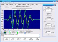
So, when you magnify the digitized waveform, you may find that it looks "chunky", more like a staircase than a ramp. Figure 1 shows an ideal low-level ramp (yellow) and the results of digitizing with inadequate bit resolution (red.) The waveform can only take on the discrete steps of the LSB size of the ADC; all information about intermediate values is lost. If you synchronously average a number of repetitions of the noise-free waveform, you get exactly the same staircase. (Note that this has nothing to do with sample rate, only the ADC resolution: Sampling faster would just mean more samples between step transitions.)
Fig. 1: Ideal and Sampled Ramp Waves
If you add noise whose peak-to-peak level is equal to the LSB resolution, you find that each step of the staircase has "grass" growing out of it, where the noise plus the signal exceeds the ADC's threshold for the next bit. Since the noise is random, the grass is different on each step and on each repetition of the waveform.
Fig. 2: Dithered Ramp, Instantaneous and Averaged
Figure 2 shows a snapshot of the sampled waveform (red) superimposed with the results of averaging 256 repetitions (yellow.) Notice that the noise causes frequent transitions in regions that were the edges of the original stairs in Figure 1, and fewer transitions near the center of each stair. It turns out that the center of each original stair is the desired true value of the ramp, which is unchanged by averaging since there are no noise-induced spikes at that point on any repetition. The noisy transition regions, on the other hand, average out to values midway between adjacent steps, forming a near-prefect replica of the original input.
To see what's going on in detail, consider that the ADC has transition points midway between each LSB step. For example, let's say this is an 8-bit ADC with an input range from 0 to 2.55 V, or 10 mV per LSB. If the input is above 5 mV but less than 15 mV, the output will have only the LSB set, indicating a 10 mV level for anything in this entire range. When the input moves above 15 mV, the ADC output reports 20 mV. Hence, without dither, we get the staircase of Figure 1.
Now consider the addition of a dither signal whose maximum excursion is +/-0.5 LSB, or +/-5 mV. Where the input ramp is exactly at 10 mV, the added noise will very rarely be at its extreme limits to bump the total above the 15 mV or below the 5 mV thresholds. Thus we see no "grass" at the center points of each bit value.
On the other hand, where the input ramp is just at the 5 mV transition point, any added noise will force the output either up to the 10 mV step or down to the 0 mV step, so we see a lot of output transitions here. If the noise has an average value of 0, we expect about half of the output values to be 10 mV and half 0, so after a lot of repetitions we expect the average output value to be pretty close to 5 mV ... even though the ADC itself can't resolve this value directly.
Similarly, intermediate values of the input ramp will produce intermediate averaged values. For example, if the ramp is at 6 mV, the ramp-plus-noise will run from 1 mV to 11 mV. Assuming a uniform distribution of noise values, we would expect about 40% of the noise values to be lower than -1 mV, such that the total input would be below 5 mV and thus the output would be 0. About 60% should be higher, giving an output of 10 mV. The average value then comes out to 6 mV, just as desired.
The improvement in resolution is proportional to the number of repetitions that are averaged together. If you average only 2 observations that are each either 0 or 10 mV, the only possible average values are 0, 5, or 10 mV. If you average 4 observations, you can get 0, 2.5, 5, 7.5, or 10 mV. Essentially, each doubling of the number of repetitions adds one bit of resolution by cutting the effective output step size in half.
There is no particular limit to this ability to increase resolution, except the practicality of how long you want to wait for the next bit. Adding an additional 8 bits of resolution only takes 256 repetitions; adding 16 bits takes 65536.
However, there is still the issue of the dither noise itself, which typically subsides as the square root of the number of repetitions averaged. Doubling the repetitions will double the resolution, but it will only cut the noise by 3 dB. Thus, the residual noise will be the limiting factor on true resolution, which improves much more slowly; you'll quickly get high apparent resolution, but the fine detail you see will just be noise until you really build up the repetitions. While the dither phenomenon may be a case where Nature finally gets generous, She's not that generous.
But that's with dither noise that is uncorrelated with itself and/or the repetition length. If you are adding dither just for the purpose of improving resolution, you can indeed get an improvement proportional to repetitions, by careful control of the dither. More on this next time.
The previous discussion also assumes noise with an amplitude of exactly +/- 0.5 LSB and a uniform distribution. If the noise level is higher, the dither process still works, but there will be a higher noise level in the averaged output. Since many real-world signals are contaminated with enough noise to require averaging simply for noise reduction, the side effect of improved resolution may be considered a pure bonus.
What about the fact that your contaminating noise may have an unknown distribution? That's not likely to be a problem unless the noise peaks are just at the +/- 0.5 LSB level. In the case where the distribution is closer to Gaussian, there might not be enough near-peak values to smooth out the transfer function as it approaches the center of each stair; effectively, this is similar to having noise with a uniform distribution but with a level that is too low. The staircase would average into a scalloped function instead of a straight line. The cure is often as simple as increasing the input gain or the noise level.
If the noise level in your signal is fairly well known, you can use that level to determine the optimum input gain for best resolution and dynamic range with a given ADC, or to determine if you need an ADC with more bits of resolution:
- If the required dynamic range is not known ahead of time, you can maximize it by setting the system gain so that the peak-to-peak noise level is the same as the LSB span. Let's say you have 1 mV of noise and an 8-bit ADC; you should set the input gain so that the ADC covers no more than a 255 mV range. If you use less gain, the noise won't be enough to provide the self-dither you need to fully resolve the true signal by averaging. More gain, on the other hand, would reduce the input range you could handle before the ADC is overdriven. To get a larger input range, you'll need an ADC with more bits: 12 bits will allow a 4095 mV range, while 16 would allow a whopping 65,535 mV.
- Alternatively, if you know the peak-to-peak range that the system must handle, divide it by the peak-to-peak noise level. That gives the approximate number of steps you need from your ADC. Round that up to the next power of 2, take the log, and divide by the log of 2. That's the number of useful ADC bits; buying an ADC with substantially more bits is overkill for this particular task.
Thus, it's always a good idea to begin with a clear vision of how the system will operate. Uninformed users have been known to specify 16-bit systems for applications where the noise spanned more than 12 of those bits, thinking that this somehow gave superior performance compared to a 12-bit or even 8-bit system. In fact, so many repetitions had to be averaged just for noise reduction, that even a 4-bit system would have given the same ultimate resolution!
Next time, we'll look at some unusual dither applications, including a single-bit ADC, DC dither, correlated dither, and pure-tone dither. In the meantime, you can experiment with dither plus averaging using the built-in signal generator of the author's Daqarta for Windows software. It turns your Windows sound card into a data acquisition system, including extensive built-in signal generation options.
All Daqarta features are free to use for 30 days or 30 sessions, after which it becomes a freeware signal generator... with full analysis capabilities. (Only the sound card inputs are ignored.)
You don't even need any external connections to the sound card to see the results of dither plus averaging visually, since you can average the raw signal before it gets to the outputs. But for a dramatic demonstration of audible dither (where your auditory system provides the averaging), you should listen to the output as you restrict the effective bits of the signal-plus-noise combination.
Previous Next
Features:
Oscilloscope
Spectrum Analyzer
8-Channel
Signal Generator
(Absolutely FREE!)
Spectrogram
Pitch Tracker
Pitch-to-MIDI
DaqMusiq Generator
(Free Music... Forever!)
Engine Simulator
LCR Meter
Remote Operation
DC Measurements
True RMS Voltmeter
Sound Level Meter
Frequency Counter
Period
Event
Spectral Event
Temperature
Pressure
MHz Frequencies
Data Logger
Waveform Averager
Histogram
Post-Stimulus Time
Histogram (PSTH)
THD Meter
IMD Meter
Precision Phase Meter
Pulse Meter
Macro System
Multi-Trace Arrays
Trigger Controls
Auto-Calibration
Spectral Peak Track
Spectrum Limit Testing
Direct-to-Disk Recording
Accessibility
Data Logger
Waveform Averager
Histogram
Post-Stimulus Time
Histogram (PSTH)
THD Meter
IMD Meter
Precision Phase Meter
Pulse Meter
Macro System
Multi-Trace Arrays
Trigger Controls
Auto-Calibration
Spectral Peak Track
Spectrum Limit Testing
Direct-to-Disk Recording
Accessibility
Applications:
Frequency response
Distortion measurement
Speech and music
Microphone calibration
Loudspeaker test
Auditory phenomena
Musical instrument tuning
Animal sound
Evoked potentials
Rotating machinery
Automotive
Product test
Contact us about
your application!
Questions? Comments? Contact us!
We respond to ALL inquiries, typically within 24 hrs.INTERSTELLAR RESEARCH:
Over 35 Years of Innovative Instrumentation
© Copyright 2007 - 2023 by Interstellar Research
All rights reserved