Another way to measure the frequency response of a linear system is to drive it with an impulse. The spectrum of the impulse response gives the frequency response of the system. The pulse must be narrow, only one sample wide, which means that not a lot of energy is delivered to the system so the response will be rather small. This may require waveform averaging to get an acceptable response signal.

In addition, the the response waveform must decay essentially to zero within the 1024 samples used to obtain the spectrum. Mechanical systems tend to have response times proportional to size, so this may not work for large, low-frequency "woofer" loudspeakers, for example.

Use the Pulse Wave option of the Generator. Set the Width Units to Samples, then set Pulse A Width to 1 sample, and Pulse B Width to 0. Make sure Pulse A Level is 100%.

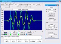
While viewing the unexpanded waveform of the output channel, set the pulse frequency low enough that you get no more than one pulse per screen. At a sample rate of 44100 Hz, that will be 43 Hz or less. Make sure Trigger is active and set to Gen Sync mode, and set the Trigger Delay to zero. You should see a single spike at the very start of the trace.

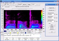
Now toggle to Spectrum mode. You will see... nothing! The energy of a single-sample pulse is spread evenly over 512 spectral lines, so each line is only 1/512 of the pulse voltage, or about 2 mV for a 1 V pulse. You will have to magnify the trace to see this, but it should be a prefectly flat line except for the 0 Hertz bin, which will be only half as big. In Y-log Spectrum mode, the line will be at about -54 dB relative to full-scale.

Important: Never use a Window function when viewing the spectrum of an impulse response or any other transient event that is completely captured in the 1024 input samples used to create the spectrum. Window functions reduce the initial portion of the response, which will seriously compromise the spectrum of the transient. Use Window functions only for continuous waveforms.

Now if you use this pulse signal to drive a speaker, you must preserve the pulse shape. This is a difficult signal for amplifiers to handle properly. The biggest danger is from "slew limiting", a form of distortion where the amplifier simply can't change its output fast enough so it (typically) produces a fixed slope at its slew limit, measured in volts/microsecond. To see if this is going to be problem for your impulse tests, use a purely resistive voltage divider to reduce the amplifier output down to a range that the sound card inputs can handle (a volt or so), and observe it directly. (See the External Gain section for a voltage divider discussion.) This way, the amplifier is still delivering its full voltage (as compared to just turning down the level) and you can see if it is behaving properly.

The input spectrum of the drive signal should be a flat line just like the output spectrum. If it's not, you'll have to decide how much error you can tolerate. If you are measuring frequency response as a production screening method, you may be able to tolerate moderate errors as long as you can still detect faulty units.

Since the speaker is being driven with a narrow, and hence low-energy, pulse, the response from the microphone may be at such a low level that it has excessive noise relative to the desired response. To clean that up, you can use synchronous waveform averaging. Once you start the Average in waveform mode, you can toggle to Spectrum mode and view the frequency response as the noise melts away. You must use Y-log Spectrum mode with User Units active and the proper Mic CAL file loaded in order to see the true speaker response. This is not strictly necessary for production screening, as long as you know what a "good" unit looks like with that microphone.

You may want to set a very large wave averager Frames Request, and then just Pause manually when there have been enough averages that the frequency response noise is acceptable.

For absolute calibration measurements, and not just relative curve shapes, you will need to boost the measured response by a factor of 512 to account for the narrow drive pulse. You can do that by reducing the External Gain setting on the Input line by that factor. If the original gain value was at the default of 1.00, set 0.00195 instead. Daqarta will interpret the actual signal as having been reduced by 512, and it will compensate by scaling up by 512 to show the true input.

See also Frequency Response Measurement

• Back to Stepped Sweep Response
• Ahead to Step Response
• Daqarta Help Contents
• Daqarta Help Index
• Daqarta Downloads
• Daqarta Home Page
• Purchase Daqarta

Questions? Comments? Contact us!