Software for Windows
Science with your Sound Card!
Features:
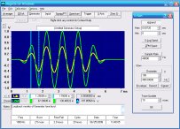
Oscilloscope
Spectrum Analyzer
8-Channel
Signal Generator
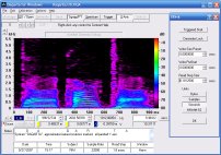
Spectrogram
Pitch Tracker
Pitch-to-MIDI
DaqMusiq Generator
(Free Music... Forever!)
Engine Simulator
LCR Meter
Remote Operation
DC Measurements
True RMS Voltmeter
Sound Level Meter
Frequency Counter
Period
Event
Spectral Event
Temperature
Pressure
MHz Frequencies
Data Logger
Waveform Averager
Histogram
Post-Stimulus Time
Histogram (PSTH)
THD Meter
IMD Meter
Precision Phase Meter
Pulse Meter
Macro System
Multi-Trace Arrays
Trigger Controls
Auto-Calibration
Spectral Peak Track
Spectrum Limit Testing
Direct-to-Disk Recording
Accessibility
Data Logger
Waveform Averager
Histogram
Post-Stimulus Time
Histogram (PSTH)
THD Meter
IMD Meter
Precision Phase Meter
Pulse Meter
Macro System
Multi-Trace Arrays
Trigger Controls
Auto-Calibration
Spectral Peak Track
Spectrum Limit Testing
Direct-to-Disk Recording
Accessibility
Applications:
Frequency response
Distortion measurement
Speech and music
Microphone calibration
Loudspeaker test
Auditory phenomena
Musical instrument tuning
Animal sound
Evoked potentials
Rotating machinery
Automotive
Product test
Contact us about
your application!
Comparing Noise Distributions
Introduction:
Auditory experiments often use broadband noise for various listening tests, and it is typically specified to have a Gaussian amplitude distribution. But can your ears tell the difference between that and a uniform White noise of the equivalent loudness? Both types of noise have the same flat frequency spectrum (they are both "white"), but the Gaussian has a much lower average amplitude for the same total dynamic range. In other words, its waveform reaches the same instantaneous peak amplitudes, but much less often.
This can make a big difference when trying to generate very loud noise, since if the system levels are set to prevent overdriving the amplifier or speakers on the peaks, the Gaussian noise will end up several dB softer. (Typically about 8 dB for the Daqarta Generator, with the Standard Deviation set to unity.)
A Gaussian noise can be created by adding multiple independent uniform sources together, so if each of those independent sources sounds the same, why should their sum sound anything other than louder?
Comparing Gaussian and Uniform White Noise:
The GausWhit.GEN setup allows you to compare two different noise sources to see if they sound qualitatively the same. It employs the general idea used in AltSine.GEN for comparing the amplitudes of two identical sine waves. Here the Left output consists of the sum of the two sources, smoothly alternating back and forth in a carefully overlapped fashion such that if they are equivalent, it will sound like one continuous source.
The two sources are separate Generator streams, each modulated by its own Burst generator. The bursts are staggered such that while one stream is falling, the other is rising. (There are no steady portions of the bursts, but that is not critical here.)
The burst parameters are set the same as in AltSine, with one critical difference: Instead of Cos^1.0, Burst Shape here uses Cos^0.5 (square root). This is because the two sources are uncorrelated, so they add in RMS fashion. Consider that when adding two identical sine waves, the result is twice the amplitude or 6 dB louder than either alone. But when adding two uncorrelated signals, only the maximum possible amplitude doubles, not the average. The result is only a 3 dB increase in loudness.
So, where the falling burst of one stream crosses the rising burst of the other, each must be only 3 dB (70.71% or the square root of 2) below the normal full-on level, rather than 50% as in AltSine. And at every other point where they overlap, the sum of the squares must be unity. The Cos^0.5 shape turns out to be exactly what is needed here.
Since the instantaneous peaks of the two streams can add to more than unity (2 * 70.71% = 141.42%), each Level control has been reduced to prevent clipping. The maximum permissible Level is the value which when multiplied by the 70.71% rise/fall midpoint gives 50%, and that value is again 70.71%. However, it is here set to a conservative 50% (-6.02 dB instead of -3 dB).
But the uniform White noise on Stream 0 has a higher average level than the Gauss noise on Stream 1, so the Stream 0 Level is reduced still further until the output sounds continuous. The proper value, found by listening tests, is about -14 dB, or 8 dB below the Gauss setting of -6 dB.
The exact value can be found by comparing long spectral averages on raw non-Burst waves at 100% Level. Load the Default.GEN setup and set the Wave type to White noise. Using Sigma cursor readout mode with Y-log (dB) mode active, set the solid and dotted cursors to cover the full unexpanded range of the spectrum (off-screen at each end). Make sure Spectrum Window is toggled off, and set the Spectrum Averager for 1024 frames.
With Wave set to White noise, the averaged value shown in the Sigma readout is -16.29 dB (relative to full scale). Toggling Wave to Gauss and repeating the average gives -24.24 dB. White is thus 7.95 dB louder than Gauss, so appying this to the GausWhit.GEN setup which has the Gauss level (Stream 1) set to -6.02 dB, the White level in Stream 0 must be 7.95 dB softer or -13.97 dB.
That value is for a Gauss noise with a Standard Deviation of 1.00; higher deviations require less reduction, and smaller deviations require more. With a deviation of 2.00 the averaged Sigma value is -18.63 dB, which is only 2.34 dB softer than White, so the White level would need to be set 2.34 below -6.02 or -8.36 dB.
Similarly, for Standard Deviation of 0.50 the averaged Sigma value is -30.27, which is 13.98 dB softer than White, so the White level would have to be 13.98 dB below -6.02 or -20.00 dB.
Comparing Gaussian and Binary White Noise:
Binary white noise is like a square wave in that is has only two states, except that it switches states at random times. It is much more efficient than uniform White or Gaussian noise at producing loud sound without overdriving a power amplifier... and even if the amplifier is driven into clipping, the output signal remains the same (assuming a "well-behaved" amplifier).
If you perform the averaged Sigma measurements discussed above, the value for binary noise turns out to be -11.53 dB... 4.76 dB louder than White (-16.29 dB) and 12.71 dB louder than Gauss (-24.24 dB).
Surprisingly, it still has a flat spectrum just like White and Gauss, and sounds exactly the same, only louder. You can demonstrate this with the GausWhit.GEN setup by toggling Stream 0 (the White source) off, and Stream 2 on. Stream 2 is actually a White source as well, but with Quantization set to 1 in the Timing dialog (opened via the button marked "Smooth TC" in the Stream 2 dialog).
A Quantization setting of 1 means that the waveform swings over its full scale in a single step. (The default 0 setting uses as many steps as the sound card can provide, which is 65536 for a 16-bit card.)
Since binary noise is 12.71 dB louder than Gauss, the Stream 2 Level is set to -18.73 dB to give the same loudness as the Gauss noise on Stream 1, which is set to -6.02 dB.
The Burst parameters are identical to the former White source on Stream 0, providing a complementary burst the "fills in the dips" of the Gauss source on Stream 1. Amazingly, you can't hear any difference in the sound or see any difference in the spectrum, but the visible waveform difference is very conspicuous.
See also Auditory Phenomena and Experiments
- Back to Zwicker Tones
- Ahead to Dither Demonstration
- Daqarta Help Contents
- Daqarta Help Index
- Daqarta Downloads
- Daqarta Home Page
- Donate to Daqarta
Questions? Comments? Contact us!
We respond to ALL inquiries, typically within 24 hrs.INTERSTELLAR RESEARCH:
Over 45 Years of Innovative Instrumentation
© Copyright 2007 - 2026 by Interstellar Research
All rights reserved